Mesh Blueprint

The Mesh Blueprint is a set of hierarchical conventions to describe mesh-based simulation data both in-memory and via files. This section provides details about the Mesh Blueprint. Lots of them.

These docs provide the main reference for all of the components of the Mesh Blueprint protocol and details about Mesh Index Protocol that are included in the Conduit Blueprint Library.

Conduit docs don’t have a Mesh Blueprint tutorial yet, if you are looking to wrap your mind around the basic mechanics of describing a mesh:

• The Ascent tutorial includes section on creating Meshes using Conduit. This is the best reference for getting started and includes C++ and Python code examples.

• The Complete Uniform Example at the end of this section shows you how to create and save a uniform grid to a file which VisIt and Ascent’s Replay utility can read.

• The Mesh Index Protocol section details functions that to generate several flavors of exemplar meshes.

Protocol

The Blueprint protocol defines a single-domain computational mesh using one or more Coordinate Sets (via child coordsets), one or more Topologies (via child topologies), zero or more Materials Sets (via child matsets), zero or more Fields (via child fields), optional Adjacency Set information (via child adjsets), and optional State information (via child state). The protocol defines multi-domain meshes as Objects that contain zero or more single-domain mesh entries.

Note

Since the multi-domain protocol accepts zero or more single-domain mesh entries, an empty Conduit Node is considered a valid multi-domain mesh. The change to accept an empty Node was introduced in Conduit 0.8.0. To check if you have a mesh with data, you can screen with dtype().is_empty(), or by using mesh blueprint property methods (i.e. number_of_domains()).

For simplicity, the descriptions below are structured relative to a single-domain mesh Object that contains one Coordinate Set named coords, one Topology named topo, and one Material Set named matset.

Coordinate Sets

To define a computational mesh, the first required entry is a set of spatial coordinate tuples that can underpin a mesh topology.

The mesh blueprint protocol supports sets of spatial coordinates from three coordinate systems:

• Cartesian: {x,y,z}

• Cylindrical: {z,r}

• Spherical: {r,theta,phi}

The mesh blueprint protocol supports three types of Coordinate Sets: uniform, rectilinear, and explicit. To conform to the protocol, each entry under coordsets must be an Object with entries from one of the cases outlined below:

• uniform

  An implicit coordinate set defined as the cartesian product of i,j,k dimensions starting at an origin (ex: {x,y,z}) using a given spacing (ex: {dx,dy,dz}).

  • Cartesian

    • coordsets/coords/type: “uniform”

    • coordsets/coords/dims/{i,j,k}

    • coordsets/coords/origin/{x,y,z} (optional, default = {0.0, 0.0, 0.0})

    • coordsets/coords/spacing/{dx,dy,dz} (optional, default = {1.0, 1.0, 1.0})

  • Cylindrical

    • coordsets/coords/type: “uniform”

    • coordsets/coords/dims/{i,j}

    • coordsets/coords/origin/{z,r} (optional, default = {0.0, 0.0})

    • coordsets/coords/spacing/{dz,dr} (optional, default = {1.0, 1.0})

  • Spherical

    • coordsets/coords/type: “uniform”

    • coordsets/coords/dims/{i,j}

    • coordsets/coords/origin/{r,theta,phi} (optional, default = {0.0, 0.0, 0.0})

    • coordsets/coords/spacing/{dr,dtheta, dphi} (optional, default = {1.0, 1.0, 1.0})

• rectilinear

  An implicit coordinate set defined as the cartesian product of passed coordinate arrays.

  • Cartesian

    • coordsets/coords/type: “rectilinear”

    • coordsets/coords/values/{x,y,z}

  • Cylindrical:

    • coordsets/coords/type: “rectilinear”

    • coordsets/coords/values/{z,r}

  • Spherical

    • coordsets/coords/type: “rectilinear”

    • coordsets/coords/values/{r,theta,phi}

• explicit

  An explicit set of coordinates, which includes values that conforms to the mcarray blueprint protocol.

  • Cartesian

    • coordsets/coords/type: “explicit”

    • coordsets/coords/values/{x,y,z}

  • Cylindrical

    • coordsets/coords/type: “explicit”

    • coordsets/coords/values/{z,r}

  • Spherical

    • coordsets/coords/type: “explicit”

    • coordsets/coords/values/{r,theta,phi}

Note

For 2D cylindrical coordinate systems we recommend specifying the Z as the first axis and R as the second axis. This matches the common expectation that Z should be displayed horizontally and R vertically in visualization tools, and that when the mesh is revolved into 3D, it will be revolved around the horizontal axis.

Note

In all of the coordinate space definitions outlined above, spherical coordinates adhere to the definitions of theta/phi used in the physics and engineering domains. Specifically, this means that theta refers to the polar angle of the coordinate (i.e. the angle from the +Z cartesian axis) and phi refers to the azimuthal angle of the coordinate (i.e. the angle from the +X cartesian axis). The figure below most succinctly describes these conventions:

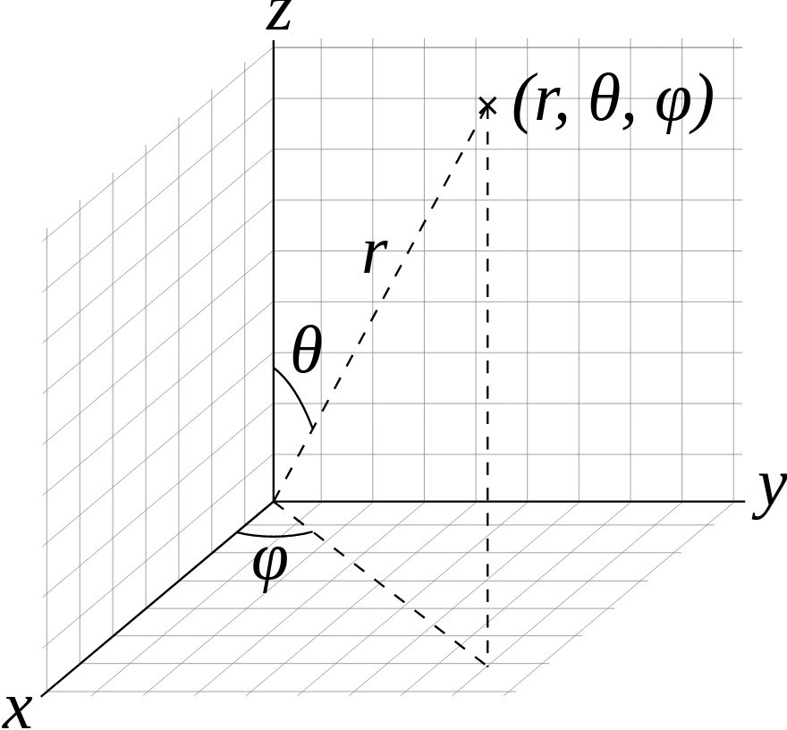
Figure of spherical coordinate conventions (courtesy of Wikipedia)

Topologies

The next entry required to describe a computational mesh is its topology. To conform to the protocol, each entry under topologies must be an Object that contains one of the topology descriptions outlined below.

Topology Nomenclature

The mesh blueprint protocol describes meshes in terms of vertices, edges, faces, and elements.

The following element shape names are supported:

Name	Geometric Type	Specified By
point	point	an index to a single coordinate tuple
line	line	indices to 2 coordinate tuples
tri	triangle	indices to 3 coordinate tuples
quad	quadrilateral	indices to 4 coordinate tuples
tet	tetrahedron	indices to 4 coordinate tuples
hex	hexahedron	indices to 8 coordinate tuples
pyramid	pyramid	indices to 5 coordinate tuples
wedge	wedge	indices to 6 coordinate tuples
polygonal	polygon	indices to N end-to-end coordinate tuples
polyhedral	polyhedron	indices to M polygonal faces
mixed	mixed	indices to coordinate tuples and/or polygonal faces

Association with a Coordinate Set

Each topology entry must have a child coordset with a string that references a valid coordinate set by name.

• topologies/topo/coordset: “coords”

Optional association with a Grid Function

Topologies can optionally include a child grid_function with a string that references a valid field by name.

• topologies/topo/grid_function: “gf”

Implicit Topology

The mesh blueprint protocol accepts four implicit ways to define a topology on a coordinate set. The first simply uses all the points in a given coordinate set and the rest define grids of elements on top of a coordinate set. For the grid cases with a coordinate set with 1D coordinate tuples, line elements are used, for sets with 2D coordinate tuples quad elements are used, and for 3D coordinate tuples hex elements are used.

• points: An implicit topology using all of the points in a coordinate set.

  • topologies/topo/coordset: “coords”

  • topologies/topo/type: “points”

• uniform: An implicit topology that defines a grid of elements on top of a uniform coordinate set.

  • topologies/topo/coordset: “coords”

  • topologies/topo/type: “uniform”

  • topologies/topo/elements/origin/{i,j,k} (optional, default = {0,0,0})

• rectilinear: An implicit topology that defines a grid of elements on top of a rectilinear coordinate set.

  • topologies/topo/coordset: “coords”

  • topologies/topo/type: “rectilinear”

  • topologies/topo/elements/origin/{i,j,k} (optional, default = {0,0,0})

• structured: An implicit topology that defines a grid of elements on top of an explicit coordinate set.

  • topologies/topo/coordset: “coords”

  • topologies/topo/type = “structured”

  • topologies/topo/elements/dims/{i,j,k}

  • topologies/topo/elements/origin/{i0,j0,k0} (optional, default = {0,0,0})

  Additional optional fields for “strided” structured:

  • topologies/topo/elements/dims/offsets: [0,0,0] (integer list 2-3 elements)

  • topologies/topo/elements/dims/strides: [i,j,k] (optional list 2-3 elements)

Structured Topology

A structured topology creates an implicitly defined topology consisting of lines, quads, or hexs, depending on the dimension of the mesh as given by the dims/i, dims/j, dims/k values. If the topology is part of a larger dataset containing multiple domains, origin values may be provided to indicate the domain’s position in the global indexing.

2D example:

coordsets:
  coords:
    type: "explicit"
    values:
      x: [0., 1., 2., 3.,
          0.1, 1.1, 2.1., 3.1,
          0.2, 1.2, 2.2, 3.2]
      y: [0., 0.1, 0., 0.1,
          1.1, 1., 1.1, 1.,
          2., 2.2, 2., 2.2]
topologies:
  mesh:
    type: "structured"
    coordset: "coords"
    elements:
      dims:
        i: 3
        j: 2

Strided Structured Topology

The elements of a structured topology will by default span all coordinates in the supplied coordset. The structured topology also supports selecting a sub-block of IJK coordinates, to create a smaller mesh without requiring the coordset’s size to be adjusted. This facilitates using existing data without having to reallocate and rearrange. This use case comes up when a host code’s data contains extra layers of elements around the mesh, which it may not be appropriate to include in the Blueprint dataset. For example, the surrounding nodes might not be initialized with sensible coordinate values.

Selecting a subset of the coordset is done by adding the elements/dims/offsets and elements/dims/strides vectors to the topology. These represent offset and stride into the supplied coordset data arrays. Both vectors contain ndims integers where ndims is the number of dimensions of the topology. Viewing the coordset data as a multi-dimensional array of size i,j(,k), the offset represents i,j(,k) indices where the selected data begin. The strides supply the number of array elements to add to the current element to move one element in I, J, or K.

The following example shows how to make a strided structured 3x2 element topology using a coordset containing 7x7 nodes.

coordsets:
  coords:
    type: "explicit"
    values:
      x: [-10.0, -6.6, -3.3, 0.0, 3.3, 6.6, 10.0,
          -10.0, -6.6, -3.3, 0.0, 3.3, 6.6, 10.0,
          -10.0, -6.6, -3.3, 0.0, 3.3, 6.6, 10.0,
          -10.0, -6.6, -3.3, 0.0, 3.3, 6.6, 10.0,
          -10.0, -6.6, -3.3, 0.0, 3.3, 6.6, 10.0,
          -10.0, -6.6, -3.3, 0.0, 3.3, 6.6, 10.0]
      y: [-10.0, -10.0, -10.0, -10.0, -10.0, -10.0, -10.0,
           -6.0, -6.0, -6.0,  -6.0,  -6.0,  -6.0, -6.0,
           -2.0, -2.0, -2.0, -2.0, -2.0, -2.0, -2.0,
            2.0, 2.0, 2.0, 2.0, 2.0, 2.0, 2.0,
            6.0, 6.0, 6.0, 6.0, 6.0, 6.0, 6.0,
            10.0, 10.0, 10.0, 10.0, 10.0, 10.0, 10.0]
topologies:
  mesh:
    type: "structured"
    coordset: "coords"
    elements:
      dims:
        i: 3
        j: 2
        # Select a subset of the coordinates
        offsets: [2, 2]  # Start at x[2][2],y[2][2]
        strides: [1, 7]  # Add 1 to move right 1
                         # Add 7 to move up 1

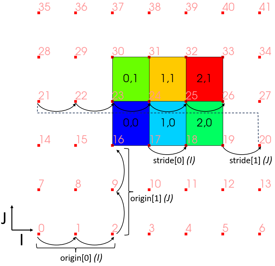
Plot of strided structured topology with coordset points shown.

When using the “strided” form of the structured topology, it may also be necessary to provide the offset, and stride values to select a subset of data from fields.

Explicit (Unstructured) Topology

Single Shape Topologies

For topologies using a homogenous collection of element shapes (eg: all hexs), the topology can be specified by a connectivity array and a shape name.

• topologies/topo/coordset: “coords”

• topologies/topo/type: “unstructured”

• topologies/topo/elements/shape: (shape name)

• topologies/topo/elements/connectivity: (index array)

Mixed Shape Toplogies

For topologies using a non-homogenous collections of element shapes (eg: hexs and tets), the topology can specified using a single shape topology for each element shape, or with the mixed shapes protocol.

• list - A Node in the List role, that contains a children that conform to the Single Shape Topology case.

• object - A Node in the Object role, that contains a children that conform to the Single Shape Topology case.

• shapes - A Node shapes that has an o2mrelation with connectivity (see below).

Element Windings

The mesh blueprint does yet not have a prescribed winding convention (a way to order the association of vertices to elements) or more generally to outline a topology’s dimensional cascade (how elements are related to faces, faces are related to edges, and edges are related to vertices. )

This is a gap we are working to solve in future versions of the mesh blueprint, with a goal of providing transforms to help convert between different winding or cascade schemes.

That said VTK (and VTK-m) winding conventions are assumed by MFEM, VisIt, VTK or Ascent when using Blueprint data.

Polygonal/Polyhedral Topologies

The polygonal and polyhedral topology shape types are structurally identical to the other explicit topology shape types (see the Single Shape Topologies section above), but the contents of their elements sections look slightly different. In particular, these sections are structured as o2mrelation objects that map elements (the ones) to their subelement constituents (the many). For polyhedral topologies, these constituents reside in an additional subelements section that specifies the polyhedral faces in a format identical to elements in a polygonal schema.

Polygonal Topologies

The schema for a polygonal shape topology is as follows:

• topologies/topo/coordset: “coords”

• topologies/topo/type: “unstructured”

• topologies/topo/elements: (o2mrelation object)

• topologies/topo/elements/shape: “polygonal”

• topologies/topo/elements/connectivity: (index array)

It’s important to note that the elements/connectivity path defines the vertex index sequences (relative to coordset) for each element in the topology. These vertex sequences must be arranged end-to-end (i.e. such that (v[i], v[i+1]) defines an edge) relative to their container polygonal elements.

The following diagram illustrates a simple polygonal topology:

#
#    4--------5
#    |`--     |
# e1 |   `.   | e0
#    |     --.|
#    7--------6
#

topologies:
  topology:
    coordset: coords
    type: unstructured
    elements:
      shape: polygonal
      connectivity: [4, 6, 5, 7, 6, 4]
      sizes: [3, 3]
      offsets: [0, 3]

Polyhedral Topologies

The schema for a polyhedral shape topology is as follows:

• topologies/topo/coordset: “coords”

• topologies/topo/type: “unstructured”

• topologies/topo/elements: (o2mrelation object)

• topologies/topo/elements/shape: “polyhedral”

• topologies/topo/elements/connectivity: (index array)

• topologies/topo/subelements: (o2mrelation object)

• topologies/topo/subelements/shape: (shape name)

• topologies/topo/subelements/connectivity: (index array)

An important nuance to the structure of a polyhedral shape topology is that the elements/connectivity path indexes into the subelements object to list the many faces associated with each one polyhedron. Similarly, the subelements/connectivity path indexes into the coordset path to list the many vertices associated with each one polyhedral face. There is no assumed ordering for constituent polyhedral faces relative to their source polyhedra.

The following diagram illustrates a simple polyhedral topology:

#
#         0
#        /|\
#       / | \ <- e0
#      /  |  \
#     /_.-3-._\
#    1.,  |  ,.4
#     \ `'2'` /
#      \  |  /
# e1 -> \ | /
#        \|/
#         5
#|

topologies:
  topology:
    coordset: coords
    type: unstructured
    elements:
      shape: polyhedral
      connectivity: [0, 1, 2, 3, 4, 0, 5, 6, 7, 8]
      sizes: [5, 5]
      offsets: [0, 5]
    subelements:
      shape: polygonal
      connectivity: [1, 2, 4, 3, 1, 2, 0, 2, 4, 0, 4, 3, 0, 3, 1, 0, 1, 2, 5, 2, 4, 5, 4, 3, 5, 3, 1, 5]
      sizes: [4, 3, 3, 3, 3, 3, 3, 3, 3]
      offsets: [0, 4, 7, 10, 13, 16, 19, 22, 25]

Mixed topologies with shapes/shape_map

The schema for a mixed shapes topology is as follows:

• topologies/topo/coordset: “coords”

• topologies/topo/coordset: “unstructured”

• topologies/topo/elements: (o2mrelation object)

• topologies/topo/elements/shape: “mixed”

• topologies/topo/elements/shape_map: (shape map node)

• topologies/topo/elements/shapes : (shapes array)

• topologies/topo/elements/sizes : (sizes array)

• topologies/topo/elements/offsets : (offsets array)

• topologies/topo/elements/connectivity : (connectivity array)

• topologies/topo/subelements: (o2mrelation object)

• topologies/topo/subelements/shape: “mixed”

• topologies/topo/subelements/shape_map: (shape map node)

• topologies/topo/subelements/shapes : (shapes array)

• topologies/topo/subelements/sizes : (sizes array)

• topologies/topo/subelements/offsets : (offsets array)

• topologies/topo/subelements/connectivity : (connectivity array)

The topologies/topo/subelements node is optional and only needed if the elements array contains polyhedra. The schemas for elements and subelements is identical and contains the following items:

shape_map, a map that relates known element type strings, e.g. “hex”, “tet” and “quad”, to numeric element types in the shapes arrray:

• shape_map/hex : (numeric entry for hexahedron, e.g. 12 - VTK_HEXAHEDRON)

• shape_map/tet : (numeric entry for tetrahedron, e.g. 10 - VTK_TETRA)

• shape_map/polyhedron : (numeric entry for polyhedron, e.g. 42 - VTK_POLYHEDRON)

• shape_map/quad : (numeric entry for quadrilateral, e.g. 9 - VTK_QUAD)

• shape_map/tri : (numeric entry for triangle, e.g. 5 - VTK_TRIANGLE)

• shape_map/polygonal: (numeric entry for polygon, e.g. 7 - VTK_POLYGON)

shapes array contains the numeric element type for each element.

sizes array contains the number of indices in the connectivity array.

connectivity array contains path the vertex index sequences (relative to coordset) for each element in the topology. In case of a polyhedral element, the indices in the connectivity array indexes into the subelements array of faces.

Note

The mixed protocol can be used to specify a mixture of element types. It is recommended that the elements of different dimensionality are not used in the same definition, unless the downstream processing code can handle this. If topologically 2D and 3D elements need to be specified, it is recommended to use two different topologies for this.

Material Sets

Materials Sets contain material name and volume fraction information defined over a specified mesh topology.

Material Set Layout Variants

Each material set conforms to a schema variant based on:

• Single or multiple buffers for volume fraction data.

• Element or material dominance.

These two choices yield four material set schema variants: multi-buffer element-dominant material sets, multi-buffer material-dominant material sets, uni-buffer element-dominant material sets, and uni-buffer material-dominant material sets.

These variants are detailed in the following sections. All of the examples in this section were created using the venn Mesh Blueprint example:

Node mesh;
int nx = 4;
int ny = 4;
float64 radius = 0.25;
std::string matset_type = "full"; // "sparse_by_element", "sparse_by_material"
conduit::blueprint::mesh::examples::venn(matset_type, nx, ny, radius, mesh);

Multi-Buffer Element-Dominant Material Sets

A multi-buffer material set is a material set variant wherein the volume fraction data is split such that one buffer exists per material. An element-dominant material set is a material set variant wherein the volume fractions and material ids are grouped by element. It is easy to fetch information grouped by element and much harder to fetch information grouped by material in an element-dominant material set.

The schema for this variant dictates that each material be presented as an Object entry of the volume_fractions field with the material name as the entry key and the material volume fractions as the entry value. Multi-buffer element-dominant material sets are a non-sparse representation, as they contain a volume fraction entry for each element.

Multi-buffer material sets also support an optional material_map, which is an Object that maps human-readable material names to unique integer material identifiers. If omitted, the map from material names to ids is inferred from the order of the material names in the volume_fractions node, with ids running from 0 to N - 1, where N is the number of materials in the material set. If the material_map is provided, children of the volume_fractions node are a subset of the children of the children of the material_map node, which is to say that a material map may reference materials for which we do not have volume fractions, but the volume fractions may not reference a material that is not present in the material map.

To conform to protocol, each matsets child of this type must be an Object that contains the following information:

• matsets/matset/topology: “topo”

• matsets/matset/volume_fractions: (object)

• matsets/matset/material_map: (optional, object with integer leaves)

The following plot and representative YAML illustrate a simple multi-buffer element-dominant material set example:

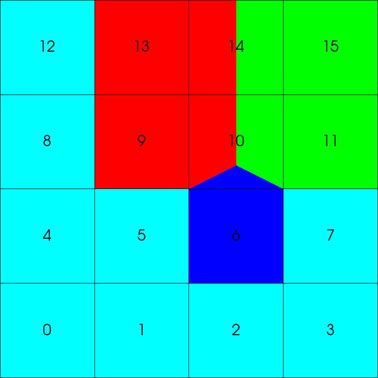
A plot of a 4x4 venn’s material boundaries with meshlines and element ids shown. Cyan represents the background, red represents circle_a, green represents circle_b, and blue represents circle_c.

matset:
  topology: "topo"
  volume_fractions:
    background: [1.0, 1.0, 1.0, 1.0, 1.0, 1.0, 0.0, 1.0, 1.0, 0.0, 0.0, 0.0, 1.0, 0.0, 0.0, 0.0]
    circle_a: [0.0, 0.0, 0.0, 0.0, 0.0, 0.0, 0.0, 0.0, 0.0, 1.0, 0.333333333333333, 0.0, 0.0, 1.0, 0.5, 0.0]
    circle_b: [0.0, 0.0, 0.0, 0.0, 0.0, 0.0, 0.0, 0.0, 0.0, 0.0, 0.333333333333333, 1.0, 0.0, 0.0, 0.5, 1.0]
    circle_c: [0.0, 0.0, 0.0, 0.0, 0.0, 0.0, 1.0, 0.0, 0.0, 0.0, 0.333333333333333, 0.0, 0.0, 0.0, 0.0, 0.0]
  material_map: # (optional)
    circle_a: 1
    circle_b: 2
    circle_c: 3
    background: 0

Again, multi-buffer element-dominant material sets are non-sparse, so they contain a volume fraction entry for each element. To find out what the volume fractions are for each material for a specific element, we simply look at values for the associated element index.

For example, for element 0, we take the 0th index of each array: background has a value of 1.0, circle_a has a value of 0.0, circle_b has a value of 0.0, and circle_c has a value of 0.0. To determine if a material is in a element, we must check that it has a nonzero volume fraction for that element. Therefore, we can infer that element 0 is 100% the background material, and the other materials are not present.

If we want to see the volume fractions for element 10, we go to the 10th index of each array: background has a value of 0.0, circle_a has a value of 0.333333333333333, circle_b has a value of 0.333333333333333, and circle_c has a value of 0.333333333333333. Therefore, we can infer that element 10 is evenly split between the circle materials and there is no background material present.

If we want to know the material ids of the materials in a specific element, we can examine the material map entry for each material in that element that has a volume fraction greater than 0.0. If no material map is present, we can infer the material id from the order of the material volume fraction arrays under the volume_fractions node.

Multi-Buffer Material-Dominant Material Sets

A multi-buffer material set is a material set variant wherein the volume fraction data is split such that one buffer exists per material. A material-dominant material set is a material set variant wherein the volume fractions and element ids are grouped by material. It is easy to fetch information grouped by material and much harder to fetch information grouped by element in a material-dominant material set.

The schema for this variant dictates that each material be presented as an Object entry of both the volume_fractions field and the element_ids field with the material name as the entry key and the material volume fractions as the entry value for the former and the per-material element ids as the latter. Multi-buffer material-dominant material sets are a sparse representation, as they only include volume fraction data for elements that have greater than 0% volume.

Multi-buffer material sets also support an optional material_map, which is an Object that maps human-readable material names to unique integer material identifiers. If omitted, the map from material names to ids is inferred from the order of the material names in the volume_fractions node, with ids running from 0 to N - 1, where N is the number of materials in the material set. If the material_map is provided, children of the volume_fractions node are a subset of the children of the children of the material_map node, which is to say that a material map may reference materials for which we do not have volume fractions, but the volume fractions may not reference a material that is not present in the material map.

To conform to protocol, each matsets child of this type must be an Object that contains the following information:

• matsets/matset/topology: “topo”

• matsets/matset/volume_fractions: (object)

• matsets/matset/element_ids: (object)

• matsets/matset/material_map: (optional, object with integer leaves)

The following plot and representative YAML illustrate a simple multi-buffer material-dominant material set example:

A plot of a 4x4 venn’s material boundaries with meshlines and element ids shown. Cyan represents the background, red represents circle_a, green represents circle_b, and blue represents circle_c.

matset:
  topology: "topo"
  volume_fractions:
    background: [1.0, 1.0, 1.0, 1.0, 1.0, 1.0, 1.0, 1.0, 1.0]
    circle_a: [1.0, 0.333333333333333, 1.0, 0.5]
    circle_b: [0.333333333333333, 1.0, 0.5, 1.0]
    circle_c: [1.0, 0.333333333333333]
  element_ids:
    background: [0, 1, 2, 3, 4, 5, 7, 8, 12]
    circle_a: [9, 10, 13, 14]
    circle_b: [10, 11, 14, 15]
    circle_c: [6, 10]
  material_map: # (optional)
    circle_a: 1
    circle_b: 2
    circle_c: 3
    background: 0

Multi-buffer material-dominant material sets are sparsely organized by material. To find out what the volume fractions are for each element for a specific material, we simply look at associated element ids and volume fractions for that material.

For example, for circle_c, we see that it is present in element 6, where it has a volume fraction of 1.0, by which we can infer that it represents the entirety of that element. We also can see that circle_c is present in element 10, where it has a volume fraction of 0.333333333333333.

If we want to know the material id for a material, we can examine the material map entry for that material. If no material map is present, we can infer the material id from the order of the material volume fraction arrays under the volume_fractions node.

Uni-Buffer Element-Dominant Material Sets

A uni-buffer material set is one that presents all of its volume fraction data in a single data buffer. An element-dominant material set is a material set variant wherein the volume fractions and material ids are grouped by element. It is easy to fetch information grouped by element and much harder to fetch information grouped by material in an element-dominant material set.

In this case, the material set schema must include a volume fraction data buffer, a parallel buffer associating each volume with a material identifier, and an Object (the material_map) that maps human-readable material names to unique integer material identifiers. Additionally, the top-level of this schema is an o2mrelation that sources from the volume fraction/material identifier buffers and targets the material topology. Uni-buffer element-dominant material sets are a sparse representation, as they only include volume fraction data for elements that have greater than 0% volume.

To conform to protocol, each matsets child of this type must be an Object that contains the following information:

• matsets/matset/topology: “topo”

• matsets/matset/material_map: (object with integer leaves)

• matsets/matset/material_ids: (integer array)

• matsets/matset/volume_fractions: (floating-point array)

As an o2mrelation, the following values may also be present:

• matsets/matset/sizes: (integer array)

• matsets/matset/offsets: (integer array)

• matsets/matset/indices: (integer array)

Note

It can help to think of how the data are traversed when understanding this structure. An element’s size and offset can be obtained by indexing the sizes and offsets with the element id. These are used to look up a tuple of data from indices. The resulting indices for the element are array indices into the material_ids and volume_fractions arrays for the current element.

The following plot and representative YAML illustrate a simple uni-buffer element-dominant material set example:

A plot of a 4x4 venn’s material boundaries with meshlines and element ids shown. Cyan represents the background, red represents circle_a, green represents circle_b, and blue represents circle_c.

matset:
  topology: "topo"
  material_map:
    circle_a: 1
    circle_b: 2
    circle_c: 3
    background: 0
  volume_fractions: [1.0, 1.0, 1.0, 1.0, 1.0, 1.0, 1.0, 1.0, 1.0, 1.0, 0.333333333333333, 0.333333333333333, 0.333333333333333, 1.0, 1.0, 1.0, 0.5, 0.5, 1.0]
  material_ids: [0, 0, 0, 0, 0, 0, 3, 0, 0, 1, 1, 2, 3, 2, 0, 1, 1, 2, 2]
  sizes: [1, 1, 1, 1, 1, 1, 1, 1, 1, 1, 3, 1, 1, 1, 2, 1]
  offsets: [0, 1, 2, 3, 4, 5, 6, 7, 8, 9, 10, 13, 14, 15, 16, 18]
  indices: [0, 1, 2, 3, 4, 5, 6, 7, 8, 9, 10, 11, 12, 13, 14, 15, 16, 17, 18] # (optional)

Again, uni-buffer element-dominant material sets are sparsely organized by element. We can use information from the o2mrelation to understand the volume_fractions and material_ids arrays.

Let’s say we want to know the material ids and volume fractions of materials in element 0. First, we examine the o2mrelation arrays. We see that our size is 1, meaning there is one material present in this element. Our offset is 0, meaning our starting index into the indices array is zero. The 0th entry in indices is also 0, meaning that the 0th values in both the volume_fractions and material_ids arrays correspond to data in element 0. If indices are not present, then we use the sizes and offsets information to get the starting index directly into the volume_fractions and material_ids arrays. If sizes and offsets are not present, then it is assumed that all sizes are 1 and offsets is a trivial prefix sum. For element 0, we see that the only material id is 0 and the volume fraction is 1.0. Looking at the material map, we can see that background is the material corresponding to material id 0. Therefore, element 0 is wholly filled with the background material.

If we want to know which materials are in element 10, we first go to the 10th index in the sizes and offsets arrays. We can see that the size is 3 and the offset is 10. Therefore, we know there are three entries in each of the volume_fractions, material_ids, and indices arrays, corresponding to three materials in element 10. The indices for element 10 are 10, 11, and 12, telling us to look in volume_fractions and material_ids at those array indices to find the relevant information. If indices were not present, then we would use offsets to find the starting index into the data arrays, and the sizes to know how many elements to read. If sizes and offsets are not present, then it is assumed that all sizes are 1 and offsets is a trivial prefix sum. For element 10, we can see that the three material ids are 1, 2, and 3, and the volume fractions are 0.333333333333333, 0.333333333333333, and 0.333333333333333. Looking at the material map, we can see that circle_a is the material corresponding to material id 1, circle_b is the material corresponding to material id 2, and circle_c is the material corresponding to material id 3. Therefore, element 10 is split evenly between the circle materials.

Here is another example showing the basic structure:

matset:
  topology: "topo"
  material_map:
    mat0: 0
    mat1: 1
    ...
  volume_fractions: [vfs_for_elem0, vfs_for_elem1, ...]
  material_ids: [mats_for_elem0, mats_for_elem1, ...]
  sizes: [number_of_mats_in_elem0, number_of_mats_in_elem1, ...]
  offsets: [offsets for the sizes]
  indices: [indirection array into the volume_fractions and material_ids]

Even though volume fractions and material ids are flattened into a single buffer, they are still grouped by element, and the o2mrelation data tells us how to interpret the uni-buffer data.

Uni-Buffer Material-Dominant Material Sets

Note

Uni-buffer material-dominant are currently unsupported in Conduit Blueprint, but it is still possible to create and reason about data in this layout. We may add support in the future as needed.

A uni-buffer material set is one that presents all of its volume fraction data in a single data buffer. A material-dominant material set is a material set variant wherein the volume fractions and element ids are grouped by material. It is easy to fetch information grouped by material and much harder to fetch information grouped by element in a material-dominant material set.

In this case, the material set schema must include a volume fraction data buffer, a parallel buffer associating each volume with an element id, and an Object (the material_map) that maps human-readable material names to unique integer material identifiers. Additionally, the top-level of this schema is an o2mrelation that sources from the volume fraction/element identifier buffers and targets the material topology. Uni-buffer material-dominant material sets are a sparse representation, as they only include volume fraction data for elements that have greater than 0% volume.

To conform to protocol, each matsets child of this type must be an Object that contains the following information:

• matsets/matset/topology: “topo”

• matsets/matset/material_map: (object with integer leaves)

• matsets/matset/element_ids: (integer array)

• matsets/matset/volume_fractions: (floating-point array)

As an o2mrelation, the following values may also be present:

• matsets/matset/sizes: (integer array)

• matsets/matset/offsets: (integer array)

• matsets/matset/indices: (integer array)

Note

It can help to think of how the data are traversed when understanding this structure. A material’s size and offset can be obtained by indexing the sizes and offsets with the material index. These are used to look up a tuple of data from indices. The resulting indices for the element are array indices into the element_ids and volume_fractions arrays for the current material.

The following plot and representative YAML illustrate a simple uni-buffer material-dominant material set example:

A plot of a 4x4 venn’s material boundaries with meshlines and element ids shown. Cyan represents the background, red represents circle_a, green represents circle_b, and blue represents circle_c.

matset:
  topology: "topo"
  material_map:
    circle_a: 1
    circle_b: 2
    circle_c: 3
    background: 0
  volume_fractions: [1.0, 0.333333333333333, 1.0, 0.5, 0.333333333333333, 1.0, 0.5, 1.0, 1.0, 0.333333333333333, 1.0, 1.0, 1.0, 1.0, 1.0, 1.0, 1.0, 1.0, 1.0]
  element_ids: [9, 10, 13, 14, 10, 11, 14, 15, 6, 10, 0, 1, 2, 3, 4, 5, 7, 8, 12]
  sizes: [4, 4, 2, 9]
  offsets: [0, 4, 8, 10]
  indices: [0, 1, 2, 3, 4, 5, 6, 7, 8, 9, 10, 11, 12, 13, 14, 15, 16, 17, 18]

Again, uni-buffer material-dominant material sets are sparsely organized by material. We can use information from the o2mrelation to understand the volume_fractions and element_ids arrays.

Let’s say we want to know the element ids and volume fractions for the first material. The first material is the first material to appear in the material map, so our first (0th) material is circle_a. First, we examine the o2mrelation arrays. We see that our size is 4, meaning there are four elements containing this material. Our offset is 0, meaning our starting index into the indices array is zero. The 0th entry in indices is also 0, meaning that the 0th values in both the volume_fractions and element_ids arrays correspond to data for the first material (circle_a). If indices are not present, then we use the sizes and offsets information to get the starting index directly into the volume_fractions and element_ids arrays. If sizes and offsets are not present, then it is assumed that all sizes are 1 and offsets is a trivial prefix sum. For circle_a, we see that the element ids are 9, 10, 13, and 14, and the volume fractions are 1.0, 0.333333333333333, 1.0, and 0.5. That means that circle_a is present in element 9 with a volume fraction of 1.0, present in element 10 with a volume fraction of 0.333333333333333, present in element 13 with a volume fraction of 1.0, and present in element 14 with a volume fraction of 0.5.

If we want to know the element ids and volume fractions for the third material, we first go to the third index in the sizes and offsets arrays. The third material is the third material to appear in the material map, so our third material is circle_c. We can see that the size is 2, meaning there are two elements containing this material. Our offset is 8, meaning our starting index into the indices array is eight. The 8th entry in indices is 8, meaning that the 8th values in both the volume_fractions and element_ids arrays correspond to data for the third material (circle_c). If indices are not present, then we use the sizes and offsets information to get the starting index directly into the volume_fractions and element_ids arrays. If sizes and offsets are not present, then it is assumed that all sizes are 1 and offsets is a trivial prefix sum. For circle_c, we see that the element ids are 6 and 10, and the volume fractions are 1.0 and 0.333333333333333. That means that circle_c is present in element 6 with a volume fraction of 1.0, present in element 10 with a volume fraction of 0.333333333333333.

Here is another example showing the basic structure:

matset:
  topology: "topo"
  material_map:
    mat0: 0
    mat1: 1
    ...
  volume_fractions: [vfs_for_mat0, vfs_for_mat1, ...]
  element_ids: [elems_for_mat0, elems_for_mat1, ...]
  sizes: [number_of_elems_mat0_is_in, number_of_elems_mat1_is_in, ...]
  offsets: [offsets for the sizes]
  indices: [indirection array into the volume_fractions and element_ids]

Even though volume fractions and element ids are flattened into a single buffer, they are still grouped by material, and the o2mrelation data tells us how to interpret the uni-buffer data.

Material Set Quick Facts

Several important details about Conduit Blueprint material sets are collected here for easy disambiguation:

• If a material_map is included, mapping human-readable material names to unique integer material identifiers, the material identifiers need not be in the range [0, N), where N is the number of materials. Material identifiers can be any set of integers. There are no restrictions on them other than that they are unique.

• In the case of multi-buffer material sets, where the volume_fractions node is an Object for which material names are the names of the children, if a material_map is included, the order of material names in the volume_fractions and in the material_map need not be the same. The volume_fractions may have less children than the material_map, but the material_map may not have less children than the volume_fractions.

• For uni-buffer material sets, the o2mrelation rules apply. Therefore, a valid uni-buffer material set may have

  • no sizes, offsets, or indices

    • for element-dominant material sets, this means that every element is assumed to have a single material present. The number of elements in volume_fractions and material_ids are the number of elements in the mesh.

    • for material-dominant material sets, this means that every material is assumed to be present in a single element. The number of elements in volume_fractions and element_ids are the number of materials in the mesh.

  • sizes and offsets, but no indices

    • for element-dominant material sets, this means that the number of materials in element i is sizes[i]. The offset into the volume_fractions and material_ids for element i is given by offsets[i].

    • for material-dominant material sets, this means that the number of elements for material i is sizes[i]. The offset into the volume_fractions and element_ids for material i is given by offsets[i].

  • indices, but no sizes nor offsets

    • for element-dominant material sets, this means that every element is assumed to have a single material present. The index into the volume_fractions and material_ids for element i is indices[i].

    • for material-dominant material sets, this means that every material is assumed to be present in a single element. The index into the volume_fractions and element_ids for material i is indices[i].

  • all three of sizes, offsets, and indices

    • for element-dominant material sets, this means that the number of materials in element i is sizes[i]. The offset into the indices for element i is given by offsets[i]. The index into the volume_fractions and material_ids for element i is indices[offsets[i]].

    • for material-dominant material sets, this means that the number of elements for material i is sizes[i]. The offset into the indices for material i is given by offsets[i]. The index into the volume_fractions and element_ids for material i is indices[offsets[i]].

• Material sets are multi-buffer if the volume_fractions child is an Object; they are uni-buffer otherwise.

• Material sets are material-dominant if they have a child called element_ids; they are element-dominant otherwise.

Material Set Tools

Conduit provides several tools for working with material sets, as working with the multiple layout specifications can be unwieldy.

The first set of tools are functions that can be used to determine what sort of material set is being worked with:

//-------------------------------------------------------------------------
bool CONDUIT_BLUEPRINT_API is_multi_buffer(const conduit::Node &matset);

//-------------------------------------------------------------------------
bool CONDUIT_BLUEPRINT_API is_uni_buffer(const conduit::Node &matset);

//-------------------------------------------------------------------------
bool CONDUIT_BLUEPRINT_API is_element_dominant(const conduit::Node &matset);

//-------------------------------------------------------------------------
bool CONDUIT_BLUEPRINT_API is_material_dominant(const conduit::Node &matset);

It is simple to ask what the layout representation is, and often code will branch like so:

// for some matset `matset`

if (is_element_dominant(matset))
{
    if (is_multi_buffer(matset))
    {
        // multi-buffer element-dominant case
    }
    else
    {
        // uni-buffer element-dominant case
    }
}
else
{
    if (is_multi_buffer(matset))
    {
        // multi-buffer material-dominant case
    }
    else
    {
        // uni-buffer material-dominant case
    }
}

The next tool in the tool box are material set conversions. A material set conforming to any of the material set layout types can be provided and converted into a material set with a different layout type:

//-------------------------------------------------------------------------
// creates a multi-buffer non-sparse case
void CONDUIT_BLUEPRINT_API to_multi_buffer_by_element(const conduit::Node &src_matset,
                                                      conduit::Node &dest_matset);

//-------------------------------------------------------------------------
// creates a uni-buffer sparse case with 1st index into elements
void CONDUIT_BLUEPRINT_API to_uni_buffer_by_element(const conduit::Node &src_matset,
                                                    conduit::Node &dest_matset,
                                                    const float64 epsilon = CONDUIT_EPSILON);

//-------------------------------------------------------------------------
// creates a multi-buffer sparse case with 1st index into materials
void CONDUIT_BLUEPRINT_API to_multi_buffer_by_material(const conduit::Node &src_matset,
                                                       conduit::Node &dest_matset,
                                                       const float64 epsilon = CONDUIT_EPSILON);
//-------------------------------------------------------------------------
// throws an error as this case is not supported
void CONDUIT_BLUEPRINT_API to_uni_buffer_by_material(const conduit::Node &src_matset,
                                                     conduit::Node &dest_matset,
                                                     const float64 epsilon = CONDUIT_EPSILON);

These are similarly simple to use:

// for some matset `matset` and some std::string `desired_matset_type`

Node converted_matset;
if (desired_matset_type == "multi-buffer-by-element")
{
    to_multi_buffer_by_element(matset, converted_matset);
}
else if (desired_matset_type == "multi-buffer-by-material")
{
    to_multi_buffer_by_material(matset, converted_matset);
}
else if (desired_matset_type == "uni-buffer-by-element")
{
    to_uni_buffer_by_element(matset, converted_matset);
}
else if (desired_matset_type == "uni-buffer-by-material")
{
    to_uni_buffer_by_material(matset, converted_matset);
}

It is also possible to convert material sets to a Silo-like mixed slot representation:

//-------------------------------------------------------------------------
// Converts a blueprint matset to the silo style sparse mixed slot 
// representation.
//
// For details about the silo format, see documentation for 
// 'DBPutMaterial' at:
// https://silo.readthedocs.io/en/latest/
void CONDUIT_BLUEPRINT_API to_silo(const conduit::Node &matset,
                                   conduit::Node &dest,
                                   const float64 epsilon = CONDUIT_EPSILON);

This will create an output with the following information:

• for matsets:

  • topology

  • material_map

  • matlist

  • mix_next

  • mix_mat

  • mix_vf

  • buffer_style

  • dominance

• for fields:

  • field_mixvar_values

  • field_values (optional)

• for specsets:

  • nmatspec

  • specnames

  • speclist

  • nmat

  • nspecies_mf

  • species_mf

  • mix_spec

  • mixlen

Conduit Blueprint also provides tools for creating/fetching material maps:

//-------------------------------------------------------------------------
// this will use set external if the matmap already exists
void CONDUIT_BLUEPRINT_API create_or_reuse_material_map(const conduit::Node &matset,
                                                        conduit::Node &material_map);
//-------------------------------------------------------------------------
// this will use set if the matmap already exists
void CONDUIT_BLUEPRINT_API create_or_copy_material_map(const conduit::Node &matset,
                                                       conduit::Node &material_map);

And tools for renumbering material ids to be in the range [0, N-1], where N is the number of materials:

//-------------------------------------------------------------------------
// renumbers material ids to run between 0 and N-1 where N is the number of
// materials.
void CONDUIT_BLUEPRINT_API renumber_material_ids(const conduit::Node &src_matset,
                                                 conduit::Node &dest_matset);
//-------------------------------------------------------------------------
// renumbers material ids to run between 0 and N-1 where N is the number of
// materials.
void CONDUIT_BLUEPRINT_API renumber_material_ids(conduit::Node &matset);

Conduit Blueprint also provides some general information methods:

//-------------------------------------------------------------------------
index_t CONDUIT_BLUEPRINT_API count_elements_from_matset(const conduit::Node &matset);
//-------------------------------------------------------------------------
index_t CONDUIT_BLUEPRINT_API count_materials_from_matset(const conduit::Node &matset);
//-------------------------------------------------------------------------
bool CONDUIT_BLUEPRINT_API is_material_in_element(const conduit::Node &matset,
                                                  const std::string &matname,
                                                  const index_t elem_id,
                                                  const float64 epsilon = CONDUIT_EPSILON);

Material Set Accessors

The problem remains that supporting all four material set layout types is cumbersome, even with helpers, converters, and information functions. It is useful to be able to walk these structures in uniform ways, which is where MatsetAccessors come into play.

The general idea with a MatsetAccessor is that it can consume a matset, a matset and a specset, a matset and a field, or all three, and it can provide data corresponding to element i and material j (and species k). MatsetAccessors know which layout type their underlying matset is and how to access information in it, abstracting away the difficulty of working with multiple material set layouts.

We can ask questions about how the MatsetAccessor was created:

// for some matset `matset`, field `field`, and specset `specset`

MatsetAccessor m_acc1 = MatsetAccessor(matset);
if (m_acc1.has_field())
    std::cout << "matset accessor 1 has field" << std::endl;
if (m_acc1.has_specset())
    std::cout << "matset accessor 1 has specset" << std::endl;

MatsetAccessor m_acc2 = MatsetAccessor(matset, field);
if (m_acc2.has_field())
    std::cout << "matset accessor 2 has field" << std::endl;
if (m_acc2.has_specset())
    std::cout << "matset accessor 2 has specset" << std::endl;

MatsetAccessor m_acc3 = MatsetAccessor(matset, specset);
if (m_acc3.has_field())
    std::cout << "matset accessor 3 has field" << std::endl;
if (m_acc3.has_specset())
    std::cout << "matset accessor 3 has specset" << std::endl;

MatsetAccessor m_acc4 = MatsetAccessor(matset, field, specset);
if (m_acc4.has_field())
    std::cout << "matset accessor 4 has field" << std::endl;
if (m_acc4.has_specset())
    std::cout << "matset accessor 4 has specset" << std::endl;

This produces the following:

matset accessor 2 has field
matset accessor 3 has specset
matset accessor 4 has field
matset accessor 4 has specset

We can also ask about general matset information:

// for some matset `matset`

MatsetAccessor m_acc = MatsetAccessor(matset);
// buffer style
bool is_uni_buffer   = m_acc.is_uni_buffer();
bool is_multi_buffer = m_acc.is_multi_buffer();

// dominance
bool is_element_dominant  = m_acc.is_element_dominant();
bool is_material_dominant = m_acc.is_material_dominant();

// number of elements
index_t num_elems = m_acc.num_elems();
// number of materials
index_t num_mats  = m_acc.num_mats();

Once we start writing loops over elements and materials, the indices of those loops matter. An element index means something different depending on what matset layout we are working with, as does a material index.

• For a multi-buffer element-dominant material set

  • elements range from 0 to the number of elements

  • materials range from 0 to the number of materials (these are material indices, not material identifiers)

  • species range from 0 to the number of species for a given material

• For a multi-buffer material-dominant material set

  • elements range from 0 to the number of elements for a given material

  • materials range from 0 to the number of materials (these are material indices, not material identifiers)

  • species range from 0 to the number of species for a given material

• For a uni-buffer element-dominant material set

  • elements range from 0 to the number of elements

  • materials range from 0 to the number of materials in a given element (these are material indices, not material identifiers)

  • species range from 0 to the number of species for a given material in a given element

• For a uni-buffer mateiral-dominant material set

  • indexing does not matter currently as this case is unsupported

Element-dominant material sets are easiest to walk by element, and material-dominant material sets are easiest to walk by material. Here is an example of walking a material set and performing data retrieval using a MatsetAccessor:

// for some matset `matset`, field `field`, and specset `specset`

MatsetAccessor m_acc = MatsetAccessor(matset, field, specset);

if (m_acc.is_element_dominant() && m_acc.is_multi_buffer())
{
    // we iterate over elements
    const index_t num_elems = m_acc.num_elems();
    for (index_t elem_idx = 0; elem_idx < num_elems; elem_idx ++)
    {
        // we ask for the total number of materials
        const index_t num_mats = m_acc.num_mats();
        for (index_t mat_idx = 0; mat_idx < num_mats; mat_idx ++)
        {
            const float64 vol_frac = m_acc.get_vol_frac(elem_idx, mat_idx);
            if (vol_frac > 0.0)
            {
                // in a multi-buffer by element matset, these values
                // only have meaning if vol_frac > 0
                const index_t mat_id = m_acc.get_mat_id(elem_idx, mat_idx);
                const index_t mat_order_id = m_acc.get_mat_order_id(elem_idx, mat_idx);
                const index_t elem_id = m_acc.get_elem_id(elem_idx, mat_idx);
                const float64 mset_val = m_acc.get_mset_val(elem_idx, mat_idx);

                const index_t num_specs_for_mat = m_acc.num_spec_for_mat(elem_idx, mat_idx);
                for (index_t spec_idx = 0; spec_idx < num_specs_for_mat; spec_idx ++)
                {
                    const float64 mf_val = m_acc.get_mass_frac(elem_idx, mat_idx, spec_idx);
                }
            }
        }
    }
}
else if (m_acc.is_material_dominant() && m_acc.is_multi_buffer())
{
    // we iterate over materials
    const index_t num_mats = m_acc.num_mats();
    for (index_t mat_idx = 0; mat_idx < num_mats; mat_idx ++)
    {
        // we ask for the number of elements for this material
        // this method is only valid for material dominant matsets
        const index_t num_elems_for_mat = m_acc.num_elems_for_mat(mat_idx);
        for (index_t elem_idx = 0; elem_idx < num_elems_for_mat; elem_idx ++)
        {
            const index_t mat_id = m_acc.get_mat_id(elem_idx, mat_idx);
            const index_t mat_order_id = m_acc.get_mat_order_id(elem_idx, mat_idx);
            const index_t elem_id = m_acc.get_elem_id(elem_idx, mat_idx);
            const float64 vol_frac = m_acc.get_vol_frac(elem_idx, mat_idx);
            const float64 mset_val = m_acc.get_mset_val(elem_idx, mat_idx);

            const index_t num_specs_for_mat = m_acc.num_spec_for_mat(elem_idx, mat_idx);
            for (index_t spec_idx = 0; spec_idx < num_specs_for_mat; spec_idx ++)
            {
                const float64 mf_val = m_acc.get_mass_frac(elem_idx, mat_idx, spec_idx);
            }
        }
    }
}
else if (m_acc.is_element_dominant() && m_acc.is_uni_buffer())
{
    // we iterate over elements
    const index_t num_elems = m_acc.num_elems();
    for (index_t elem_idx = 0; elem_idx < num_elems; elem_idx ++)
    {
        // we ask for the number of materials in this element
        // this method is only valid for sparse element dominant matsets
        const index_t num_mats_for_elem = m_acc.num_mats_for_elem(elem_idx);
        for (index_t mat_idx = 0; mat_idx < num_mats_for_elem; mat_idx ++)
        {
            const index_t mat_id = m_acc.get_mat_id(elem_idx, mat_idx);
            const index_t mat_order_id = m_acc.get_mat_order_id(elem_idx, mat_idx);
            const index_t elem_id = m_acc.get_elem_id(elem_idx, mat_idx);
            const float64 vol_frac = m_acc.get_vol_frac(elem_idx, mat_idx);
            const float64 mset_val = m_acc.get_mset_val(elem_idx, mat_idx);

            const index_t num_specs_for_mat = m_acc.num_spec_for_mat(elem_idx, mat_idx);
            for (index_t spec_idx = 0; spec_idx < num_specs_for_mat; spec_idx ++)
            {
                const float64 mf_val = m_acc.get_mass_frac(elem_idx, mat_idx, spec_idx);
            }
        }
    }
}
else // (m_acc.is_material_dominant() && m_acc.is_uni_buffer())
{
    CONDUIT_ERROR("Currently unsupported case.");
}

When walking by materials either in an inner or an outer loop, what does the mat_idx represent?

• If walking in an outer loop, the mat_idx iterates over the materials in the order they appear in the material_map, if it is present. If it is not present, then the matset must be multi-buffer, so the order of materials is the order in which they appear as children under the volume_fractions node.

• If walking in an inner loop, then it depends on the material set layout. For multi-buffer material sets, this order is always the order the materials appear in the matset, as discussed in the previous bullet. For uni-buffer element-dominant material sets, the order of materials is the order in which they appear in a given element.

Fields

Fields are used to hold simulation state arrays associated with a mesh topology and (optionally) a mesh material set.

Each field entry can define an mcarray of material-independent values and/or an mcarray of per-material values. These data arrays must be specified alongside a source space, which specifies the space over which the field values are defined (i.e. a topology for material-independent values and a material set for material-dependent values). Minimally, each field entry must specify one of these data sets, the source space for the data set, an association type (e.g. per-vertex, per-element, or per-grid-function-entity), and a volume scaling type (e.g. volume-dependent, volume-independent). Thus, to conform to protocol, each entry under the fields section must be an Object that adheres to one of the following descriptions:

• Material-Independent Fields:

  • fields/field/association: “vertex” | “element”

  • fields/field/basis: (mfem-style finite element collection name) (replaces “association”)

  • fields/field/volume_dependent: “true” | “false”

  • fields/field/topology: “topo”

  • fields/field/values: (mcarray)

  • fields/field/offsets: (integer array) (optional - for strided structured topology)

  • fields/field/strides: (integer array) (optional - for strided structured topology)

• Material-Dependent Fields:

  • fields/field/association: “vertex” | “element”

  • fields/field/basis: (mfem-style finite element collection name) (replaces “association”)

  • fields/field/volume_dependent: “true” | “false”

  • fields/field/matset: “matset”

  • fields/field/matset_values: (mcarray)

• Mixed Fields:

  • fields/field/association: “vertex” | “element”

  • fields/field/basis: (mfem-style finite element collection name) (replaces “association”)

  • fields/field/volume_dependent: “true” | “false”

  • fields/field/topology: “topo”

  • fields/field/values: (mcarray)

  • fields/field/matset: “matset”

  • fields/field/matset_values: (mcarray)

Topology Association for Field Values

For implicit topologies, the field values are associated with the topology by fast varying logical dimensions starting with i, then j, then k.

For explicit topologies, the field values are associated with the topology by assuming the order of the field values matches the order the elements are defined in the topology.

Strided Structured Fields

When creating structured topologies for mesh data that is surrounded by unwanted extra layers, a structured topology can provide offsets and strides to indicate that Blueprint should ignore the extra layers of data. This lets the topology be represented without having to rearrange any of the coordset data. The same issue arises for fields so Blueprint allows fields to supply offsets and strides to select a subset of a larger array.

The following example is for a mesh that supplied 7x7 actual nodes in the coordset but only defined a 3x2 element, or 4x3 node topology defined over a subset of the nodes. The offsets and strides values in the field are used to select a subset of the field values, which in reality would be supplied in-memory from a host code’s data structures. For readability, the values selected using offsets` and strides are non-zero while unselected values are zero.

fields:
  vert_vals:
    association: "vertex"
    topology: "mesh"
    offsets: [2, 2]
    strides: [1, 7]
    values: [0.0, 0.0, 0.0, 0.0, 0.0, 0.0, 0.0,
             0.0, 0.0, 0.0, 0.0, 0.0, 0.0, 0.0,
             0.0, 0.0, 1.0, 2.0, 3.0, 4.0, 0.0,
             0.0, 0.0, 5.0, 6.0, 7.0, 8.0, 0.0,
             0.0, 0.0, 9.0, 10.0, 11.0, 12.0, 0.0,
             0.0, 0.0, 0.0, 0.0, 0.0, 0.0, 0.0]

Species Sets

Species Sets are a means of representing multi-dimensional per-material quantities, most commonly per-material substance fractions.

Individual Species Sets are entries in the specsets section of the Blueprint hierarchy, and these entries are formatted in much the same way as fields entries that describe per-material, multi-dimensional fields. Just as with this class of fields entries, each specsets entry must specify the material set over which it is defined and enumerate its values within an mcarray that’s organized first by materials (shallower level of nesting) and then by species components (deeper level of nesting). To put it in short, each entry in the specsets section of the Blueprint hierarchy must be an Object that follows this template:

• specsets/specset/matset: “matset”

• specsets/specset/matset_values: (mcarray)

Nesting Sets

Nesting Sets are used to represent the nesting relationships between different domains in multi-domain mesh environments. Most commonly, this subset of the Blueprint specification is used for AMR (adaptive mesh refinement) meshes.

Each entry in the Nesting Sets section contains an independent set of nesting relationships between domains in the described mesh. On an individual basis, a nesting set contains a source topology, an element association, and a list of nesting windows. The windows for a particular nesting set describe the topological nesting pattern for a paired set of domains, which includes the ID of the partnered domain, the type of the partnered domain (parent or child), the per-dimension zone ratios of this domain relative to the partnered domain, and the self-relative dimensions and origin (provided in terms of local domain coordinates) of the nesting relationship. The Blueprint schema for each entry in the nestsets section matches the following template:

• nestsets/nestset/association: “vertex” | “element”

• nestsets/nestset/topology: “topo”

• nestsets/nestset/windows/window/domain_id: (integer)

• nestsets/nestset/windows/window/domain_type: “parent” | “child”

• nestsets/nestset/windows/window/ratio/{i, j, k}

• nestsets/nestset/windows/window/origin/{i, j, k}

• nestsets/nestset/windows/window/dims/{i, j, k}

Note

Many structured AMR codes use global coordinate identifiers when specifying each window’s origin. Such coordinates must be transformed to domain-local coordinates to be Blueprint-compliant. Given the global structured origin of a window’s associated topology topo_origin (which isn’t in the Blueprint, but is likely stored somewhere in the client code), the global origin can be transformed into a local origin like so:

// 'window_origin': starts out as a global index, but is transformed into
// a domain-local index through this procedure
conduit::Node &window_origin = // path to nestset/windows/window/origin
conduit::Node &topo_origin = // loaded from client code; {i, j, k} structure

conduit::NodeIterator origin_it = window_origin.children();
while(origin_it.has_next())
{
    conduit::Node &window_dim = origin_it.next();
    conduit::Node &topo_dim = topo_origin[origin_it.name()];

    conduit::int64 new_dim_val = window_dim.to_int64() - topo_dim.to_int64();
    conduit::Node &new_dim(conduit::DataType::int64(1), &new_dim_val, true);
    new_dim.to_data_type(window_dim.dtype().id(), window_dim);
}

Each domain that contains a Nesting Sets section must also update its State section to include the domain’s global nesting level. This additional requirement adds the follow constraint to the state section:

• state/level_id: (integer)

Note

The Nesting Sets section currently only supports nesting specifications for structured topologies. There are plans to extend this feature to support unstructured topologies in future versions of Conduit.

Adjacency Sets

Adjacency Sets are used to outline the shared geometry between subsets of domains in multi-domain meshes.

Each entry in the Adjacency Sets section is meant to encapsulate a set of adjacency information shared between domains. Each individual adjacency set contains a source topology, an element association, and a list of adjacency groups. An adjacency set’s contained groups describe adjacency information shared between subsets of domains, which is represented by a subset of adjacent neighbor domains IDs and a list of shared element IDs. The fully-defined Blueprint schema for the adjsets entries looks like the following:

• adjsets/adjset/association: “vertex” | “element”

• adjsets/adjset/topology: “topo”

• adjsets/adjset/groups/group/neighbors: (integer array)

• adjsets/adjset/groups/group/values: (integer array)

It’s important to note that the groups in an Adjacency Set associate across domains based on their names (e.g. domain0/adjsets/adjset/groups/1 will be associated with domain*/adjsets/adjset/groups/1). For data publishers that are agnostic about group names, the conduit::blueprint::mesh::utils::adjset::canonicalize utility method can be used to assign cross-domain matching names:

conduit::Node &unidomain_mesh = // loaded from the client code
conduit::Node &unidomain_adjset = unidomain_mesh["adjsets"].child(0);
conduit::Node &unidomain_domid = unidomain_mesh["state/domain_id"];

unidomain_domid.print();
// > 0
unidomain_adjset["groups"].print();
// > a:
// >   neighbors: [1, 2, 3]
// >   values: [...]
// > b:
// >   neighbors: [1]
// >   values: [...]
// > c:
// >   neighbors: [2]
// >   values: [...]

conduit::bleuprint::mesh::utils::adjset::canonicalize(unidomain_adjset);

unidomain_adjset["groups"].print();
// > group_0_1_2_3:
// >   neighbors: [1, 2, 3]
// >   values: [...]
// > group_0_1:
// >   neighbors: [1]
// >   values: [...]
// > group_0_2:
// >   neighbors: [2]
// >   values: [...]

Adjacency Set Variants

There’s a great deal of flexibility in how the adjacency groups of an Adjacency Set can be constructed. Blueprint Mesh contains detection and transformation functions for the most commonly targeted formats. The two variants currently supported are pairwise and max-share.

Pairwise Adjacency Sets

A pairwise adjacency set is one that contains groups that represent the relationship between the host domain and a single neighboring domain (i.e. domain “pairs”).

The following diagram illustrates a simple pairwise material set example:

#  domain0    domain1
# +--------++--------+
# |     v01||v11     |
# |        ||        |
# |     v00||v10     |
# +--------++--------+
# +--------+
# |     v20|
# |        |
# |     v21|
# +--------+
#  domain2

domain0:
  state:
    domain_id: 0
  adjsets:
    adjset:
      association: vertex
      topology: topology
      groups:
        domain_0_1:
          neighbors: [1]
          values: [v00, v01]
        domain_0_2:
          neighbors: [2]
          values: [v00]

Max-Share Adjacency Sets

A max-share adjacency set is one with groups that “maximally share” index data. In other words, these adjacency sets present index data so that it isn’t duplicated between groups.

The following diagram illustrates a simple max-share material set example:

#  domain0    domain1
# +--------++--------+
# |     v01||v11     |
# |        ||        |
# |     v00||v10     |
# +--------++--------+
# +--------+
# |     v20|
# |        |
# |     v21|
# +--------+
#  domain2

domain0:
  state:
    domain_id: 0
  adjsets:
    adjset:
      association: vertex
      topology: topology
      groups:
        domain_0_1_2:
          neighbors: [1, 2]
          values: [v00]
        domain_0_1:
          neighbors: [1]
          values: [v01]

State

Optional state information is used to provide metadata about the mesh. While the mesh blueprint is focused on describing a single domain of a domain decomposed mesh, the state info can be used to identify a specific mesh domain in the context of a domain decomposed mesh.

To conform, the state entry must be an Object and can have the following optional entries:

• state/time: (number)

• state/cycle: (number)

• state/domain_id: (integer)

Mesh Index Protocol

It is common for Blueprint data files to represent meshes that have been partitioned and must later be treated as a whole. Blueprint root files contain an index that facilitates reading in many individual Blueprint files. Blueprint root files contain metadata about the overall contents of individual files as well as hints for constructing filenames that make up the whole Blueprint dataset. An analysis tool can load the root file and know which individual files comprise the dataset and information about the data contained therein. While Blueprint provides high level functions for saving and loading files, some of which automatically create the root file, it is sometimes necessary to know the structure.

• blueprint_index/<meshname>/coordsets

• blueprint_index/<meshname>/topologies

• blueprint_index/<meshname>/fields

• blueprint_index/<meshname>/state

The root file is a hierarchical index dataset created with Conduit that has been saved to a file using Relay. The root file must contain a blueprint_index node under which multiple named mesh nodes can be created. There must be at least one mesh node. The contents under the mesh node consist of metadata that mirror the structure of a typical Blueprint dataset, with “coordsets”, “topologies”, “fields”, and “state” nodes. Rather than providing actual data in these nodes, they include “path” nodes that specify the path to their corresponding structures in the individual Blueprint data files. Fields can supply an optional “display_name” string that can rename the field in VisIt, which can be used to group related fields. Mesh index metadata can be created using the conduit::blueprint::mpi::mesh::generate_index() function when passed a valid Blueprint dataset.

• blueprint_index/<meshname>/fields/<fieldname>/number_of_components: {number 1 or 3)

• blueprint_index/<meshname>/fields/<fieldname>/topology: (string)

• blueprint_index/<meshname>/fields/<fieldname>/association: vertex|element

• blueprint_index/<meshname>/fields/<fieldname>/path: (string)

• blueprint_index/<meshname>/fields/<fieldname>/display_name: (optional string)

Finally, the Blueprint index contains several nodes that provide the information needed to generate filenames and locate data within other files. The “file_pattern” value provides a filename template with wildcards that is used to generate filenames. Wildcards follow C-Language printf() format string conventions for integers (e.g. “%05d”). Wildcards are substituted with integers in the range of [0, number_of_files] where number_of_files is provided by the “number_of_files” node. In addition, metadata about the protocol used for individual Blueprint data files is provided using “protocol/name” and “protocol/version”.

• number_of_files: (number)

• file_pattern: (string)

• number_of_trees: (number)

• tree_pattern: (string, default = “/”)

• protocol/name: (string)

• protocol/version: (string)

Example of a Basic Root File:

blueprint_index:
  mesh: # Most entries under here were generated using generate_index()
    state:
      cycle: 100
      time: 3.1415
      path: "state"
      number_of_domains: 4
    coordsets:
      coords:
        type: "uniform"
        coord_system:
          axes:
            x:
            y:
            z:
          type: "cartesian"
        path: "coordsets/coords"
    topologies:
      mesh:
        type: "uniform"
        coordset: "coords"
        path: "topologies/mesh"
    fields:
      density_000:
        number_of_components: 1
        topology: "mesh"
        association: "vertex"
        path: "fields/density_000"
        display_name: "density/mat0" # NOTE: This renames the field in VisIt
      density_001:
        number_of_components: 1
        topology: "mesh"
        association: "vertex"
        path: "fields/density_001"
        display_name: "density/mat1"
# These entries specify the number and names of the files that make up the dataset.
number_of_files: 4
file_pattern: "bp/bp_%05d.hdf5"
number_of_trees: 4
tree_pattern: "/"
protocol:
  name: "hdf5"
  version: "0.4.0"

Example code:

// Call on each of 4 MPI ranks.
conduit::Node mesh, bp_index;
conduit::blueprint::mesh::examples::braid("uniform", 10, 10, 10, mesh);
char domainFile[1024];
sprintf(domainFile, "./bp/bp_%04d.hdf5", rank);
conduit::relay::io::save(mesh, domainFile, "hdf5");

conduit::blueprint::mpi::mesh::generate_index(mesh,
                                              "",
                                              bp_index["blueprint_index/mesh"],
                                              MPI_COMM_WORLD);
bp_index["file_pattern"] = "./bp/bp_%04d.hdf5";
bp_index["number_of_files"] = 4;
bp_index["number_of_trees"] = 4;
bp_index["protocol/name"] = "hdf5";
bp_index["protocol/version"] = "0.4.0";
bp_index["tree_pattern"] = "/";
if(rank == 0)
    conduit::relay::io::save(bp_index, "bp.root", "hdf5");

Root files are needed to read Blueprint data into tools such as VisIt. At present, VisIt imposes a few caveats when reading Blueprint data:

• A root file is always required.

• The root file must be saved to hdf5, json, or yaml protocols.

• Individual Blueprint files that contain actual data may use hdf5, json, or yaml protocols as long as the protocol matches the index’s “protocol/name” value.

• If fields supply a display_name string then that name will be used instead of the field name. (e.g. display_name: “menu1/menu2/fieldname”)

Mesh Blueprint Examples

The C++ conduit::blueprint::mesh::examples namespace and the Python conduit.blueprint.mesh.examples module provide functions that generate example Mesh Blueprint data. For details on how to write these data sets to files, see the unit tests that exercise these examples in src/tests/blueprint/t_blueprint_mesh_examples.cpp and the mesh output example below. This section outlines the examples that demonstrate the most commonly used mesh schemas.

basic

The simplest of the mesh examples, basic(), generates an homogenous example mesh with a configurable element representation/type (see the mesh_type table below) spanned by a single scalar field that contains a unique identifier for each mesh element. The function that needs to be called to generate an example of this type has the following signature:

conduit::blueprint::mesh::examples::basic(const std::string &mesh_type, // element type/dimensionality
                                          index_t nx,                   // number of grid points along x
                                          index_t ny,                   // number of grid points along y
                                          index_t nz,                   // number of grid points along z (3d only)
                                          Node &res);                   // result container

The element representation, type, and dimensionality are all configured through the mesh_type argument. The supported values for this parameter and their corresponding effects are outlined in the table below:

Mesh Type	Dimensionality	Coordset Type	Topology Type	Element Type
uniform	2d/3d	implicit	implicit	quad/hex
rectilinear	2d/3d	implicit	implicit	quad/hex
structured	2d/3d	explicit	implicit	quad/hex
tris	2d	explicit	explicit	tri
quads	2d	explicit	explicit	quad
polygons	2d	explicit	explicit	polygon
tets	3d	explicit	explicit	tet
hexs	3d	explicit	explicit	hex
wedges	3d	explicit	explicit	wedge
pyramids	3d	explicit	explicit	pyramid
polyhedra	3d	explicit	explicit	polyhedron

The remainder of this section demonstrates each of the different basic() mesh types, outlining each type with a simple example that (1) presents the generating call, (2) shows the results of the call in Blueprint schema form, and (3) displays the corresponding graphical rendering of this schema.

Uniform

• Usage Example

// create container node
Node mesh;
// generate simple uniform 2d 'basic' mesh
conduit::blueprint::mesh::examples::basic("uniform", 3, 3, 0, mesh);
// print out results
std::cout << mesh.to_yaml() << std::endl;

• Result

coordsets: 
  coords: 
    type: "uniform"
    dims: 
      i: 3
      j: 3
    origin: 
      x: -10.0
      y: -10.0
    spacing: 
      dx: 10.0
      dy: 10.0
topologies: 
  mesh: 
    type: "uniform"
    coordset: "coords"
fields: 
  field: 
    association: "element"
    topology: "mesh"
    volume_dependent: "false"
    values: [0.0, 1.0, 2.0, 3.0]

• Visual

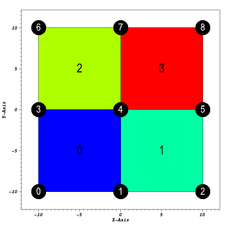
Pseudocolor plot of basic (mesh type ‘uniform’)

Rectilinear

• Usage Example

// create container node
Node mesh;
// generate simple rectilinear 2d 'basic' mesh
conduit::blueprint::mesh::examples::basic("rectilinear", 3, 3, 0, mesh);
// print out results
std::cout << mesh.to_yaml() << std::endl;

• Result

coordsets: 
  coords: 
    type: "rectilinear"
    values: 
      x: [-10.0, 0.0, 10.0]
      y: [-10.0, 0.0, 10.0]
topologies: 
  mesh: 
    type: "rectilinear"
    coordset: "coords"
fields: 
  field: 
    association: "element"
    topology: "mesh"
    volume_dependent: "false"
    values: [0.0, 1.0, 2.0, 3.0]

• Visual

Pseudocolor plot of basic (mesh type ‘rectilinear’)

Structured

• Usage Example

// create container node
Node mesh;
// generate simple structured 2d 'basic' mesh
conduit::blueprint::mesh::examples::basic("structured", 3, 3, 1, mesh);
// print out results
std::cout << mesh.to_yaml() << std::endl;

• Result

coordsets: 
  coords: 
    type: "explicit"
    values: 
      x: [-10.0, 0.0, 10.0, -10.0, 0.0, 10.0, -10.0, 0.0, 10.0]
      y: [-10.0, -10.0, -10.0, 0.0, 0.0, 0.0, 10.0, 10.0, 10.0]
topologies: 
  mesh: 
    type: "structured"
    coordset: "coords"
    elements: 
      dims: 
        i: 2
        j: 2
fields: 
  field: 
    association: "element"
    topology: "mesh"
    volume_dependent: "false"
    values: [0.0, 1.0, 2.0, 3.0]

• Visual

Pseudocolor plot of basic (mesh type ‘structured’)

Tris

• Usage Example

// create container node
Node mesh;
// generate simple explicit tri-based 2d 'basic' mesh
conduit::blueprint::mesh::examples::basic("tris", 3, 3, 0, mesh);
// print out results
std::cout << mesh.to_yaml() << std::endl;

• Result

coordsets: 
  coords: 
    type: "explicit"
    values: 
      x: [-10.0, 0.0, 10.0, -10.0, 0.0, 10.0, -10.0, 0.0, 10.0]
      y: [-10.0, -10.0, -10.0, 0.0, 0.0, 0.0, 10.0, 10.0, 10.0]
topologies: 
  mesh: 
    type: "unstructured"
    coordset: "coords"
    elements: 
      shape: "tri"
      connectivity: [0, 3, 4, 0, 1, 4, 1, 4, 5, 1, 2, 5, 3, 6, 7, 3, 4, 7, 4, 7, 8, 4, 5, 8]
fields: 
  field: 
    association: "element"
    topology: "mesh"
    volume_dependent: "false"
    values: [0.0, 1.0, 2.0, 3.0, 4.0, 5.0, 6.0, 7.0]

• Visual

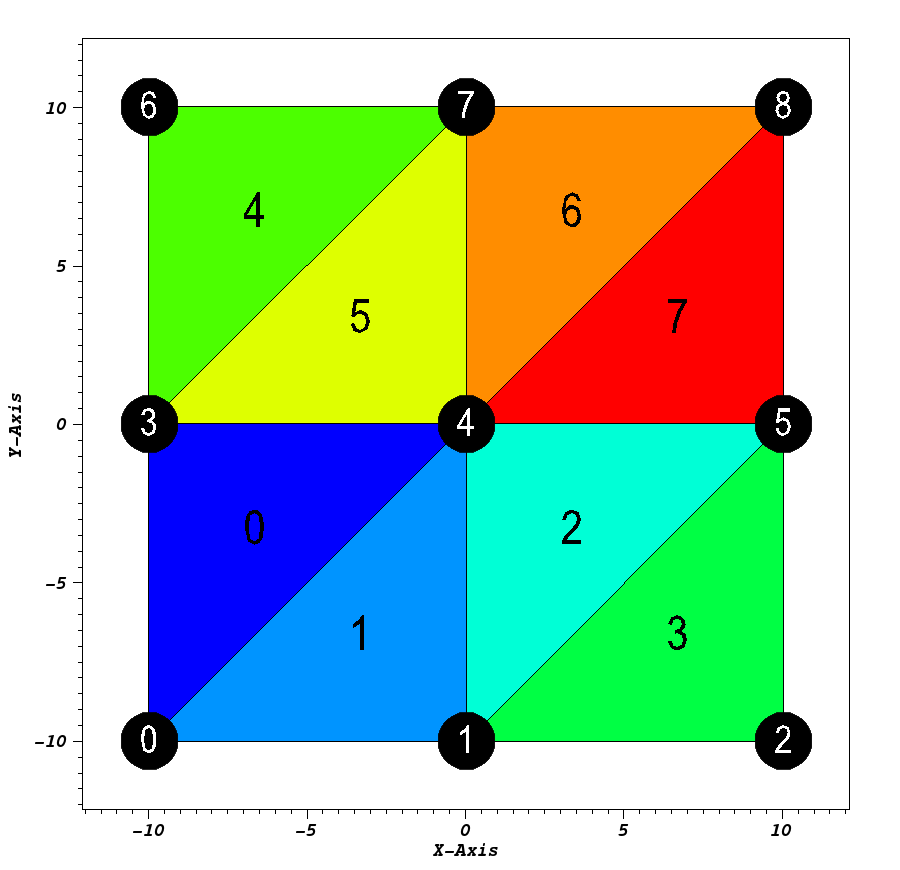
Pseudocolor plot of basic (mesh type ‘tris’)

Quads

• Usage Example

// create container node
Node mesh;
// generate simple explicit quad-based 2d 'basic' mesh
conduit::blueprint::mesh::examples::basic("quads", 3, 3, 0, mesh);
// print out results
std::cout << mesh.to_yaml() << std::endl;

• Result

coordsets: 
  coords: 
    type: "explicit"
    values: 
      x: [-10.0, 0.0, 10.0, -10.0, 0.0, 10.0, -10.0, 0.0, 10.0]
      y: [-10.0, -10.0, -10.0, 0.0, 0.0, 0.0, 10.0, 10.0, 10.0]
topologies: 
  mesh: 
    type: "unstructured"
    coordset: "coords"
    elements: 
      shape: "quad"
      connectivity: [0, 3, 4, 1, 1, 4, 5, 2, 3, 6, 7, 4, 4, 7, 8, 5]
fields: 
  field: 
    association: "element"
    topology: "mesh"
    volume_dependent: "false"
    values: [0.0, 1.0, 2.0, 3.0]

• Visual

Pseudocolor plot of basic (mesh type ‘quads’)

Polygons

• Usage Example

// create container node
Node mesh;
// generate simple explicit poly-based 2d 'basic' mesh
conduit::blueprint::mesh::examples::basic("polygons", 3, 3, 0, mesh);
// print out results
std::cout << mesh.to_yaml() << std::endl;

• Result

coordsets: 
  coords: 
    type: "explicit"
    values: 
      x: [-10.0, 0.0, 10.0, -10.0, 0.0, 10.0, -10.0, 0.0, 10.0]
      y: [-10.0, -10.0, -10.0, 0.0, 0.0, 0.0, 10.0, 10.0, 10.0]
topologies: 
  mesh: 
    type: "unstructured"
    coordset: "coords"
    elements: 
      shape: "polygonal"
      connectivity: [0, 3, 4, 1, 1, 4, 5, 2, 3, 6, 7, 4, 4, 7, 8, 5]
      sizes: [4, 4, 4, 4]
      offsets: [0, 4, 8, 12]
fields: 
  field: 
    association: "element"
    topology: "mesh"
    volume_dependent: "false"
    values: [0.0, 1.0, 2.0, 3.0]

• Visual

Pseudocolor plot of basic (mesh type ‘polygons’)

Tets

• Usage Example

// create container node
Node mesh;
// generate simple explicit tri-based 3d 'basic' mesh
conduit::blueprint::mesh::examples::basic("tets", 3, 3, 3, mesh);
// print out results
std::cout << mesh.to_yaml() << std::endl;

• Result

coordsets: 
  coords: 
    type: "explicit"
    values: 
      x: [-10.0, 0.0, 10.0, -10.0, 0.0, 10.0, -10.0, 0.0, 10.0, -10.0, 0.0, 10.0, -10.0, 0.0, 10.0, -10.0, 0.0, 10.0, -10.0, 0.0, 10.0, -10.0, 0.0, 10.0, -10.0, 0.0, 10.0]
      y: [-10.0, -10.0, -10.0, 0.0, 0.0, 0.0, 10.0, 10.0, 10.0, -10.0, -10.0, -10.0, 0.0, 0.0, 0.0, 10.0, 10.0, 10.0, -10.0, -10.0, -10.0, 0.0, 0.0, 0.0, 10.0, 10.0, 10.0]
      z: [-10.0, -10.0, -10.0, -10.0, -10.0, -10.0, -10.0, -10.0, -10.0, 0.0, 0.0, 0.0, 0.0, 0.0, 0.0, 0.0, 0.0, 0.0, 10.0, 10.0, 10.0, 10.0, 10.0, 10.0, 10.0, 10.0, 10.0]
topologies: 
  mesh: 
    type: "unstructured"
    coordset: "coords"
    elements: 
      shape: "tet"
      connectivity: [0, 4, 1, 13, 0, 3, 4, 13, 0, 12, 3, 13, 0, 9, 12, 13, 0, 10, 9, 13, 0, 1, 10, 13, 1, 5, 2, 14, 1, 4, 5, 14, 1, 13, 4, 14, 1, 10, 13, 14, 1, 11, 10, 14, 1, 2, 11, 14, 3, 7, 4, 16, 3, 6, 7, 16, 3, 15, 6, 16, 3, 12, 15, 16, 3, 13, 12, 16, 3, 4, 13, 16, 4, 8, 5, 17, 4, 7, 8, 17, 4, 16, 7, 17, 4, 13, 16, 17, 4, 14, 13, 17, 4, 5, 14, 17, 9, 13, 10, 22, 9, 12, 13, 22, 9, 21, 12, 22, 9, 18, 21, 22, 9, 19, 18, 22, 9, 10, 19, 22, 10, 14, 11, 23, 10, 13, 14, 23, 10, 22, 13, 23, 10, 19, 22, 23, 10, 20, 19, 23, 10, 11, 20, 23, 12, 16, 13, 25, 12, 15, 16, 25, 12, 24, 15, 25, 12, 21, 24, 25, 12, 22, 21, 25, 12, 13, 22, 25, 13, 17, 14, 26, 13, 16, 17, 26, 13, 25, 16, 26, 13, 22, 25, 26, 13, 23, 22, 26, 13, 14, 23, 26]
fields: 
  field: 
    association: "element"
    topology: "mesh"
    volume_dependent: "false"
    values: [0.0, 1.0, 2.0, 3.0, 4.0, 5.0, 6.0, 7.0, 8.0, 9.0, 10.0, 11.0, 12.0, 13.0, 14.0, 15.0, 16.0, 17.0, 18.0, 19.0, 20.0, 21.0, 22.0, 23.0, 24.0, 25.0, 26.0, 27.0, 28.0, 29.0, 30.0, 31.0, 32.0, 33.0, 34.0, 35.0, 36.0, 37.0, 38.0, 39.0, 40.0, 41.0, 42.0, 43.0, 44.0, 45.0, 46.0, 47.0]

• Visual

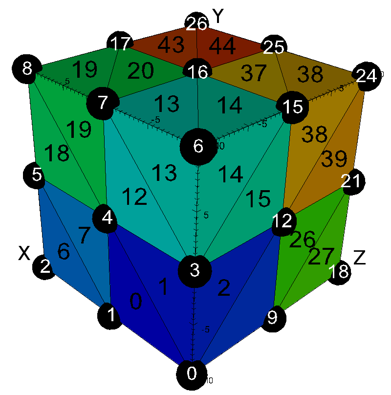
Pseudocolor plot of basic (mesh type ‘tets’)

Hexs

• Usage Example

// create container node
Node mesh;
// generate simple explicit quad-based 3d 'basic' mesh
conduit::blueprint::mesh::examples::basic("hexs", 3, 3, 3, mesh);
// print out results
std::cout << mesh.to_yaml() << std::endl;

• Result

coordsets: 
  coords: 
    type: "explicit"
    values: 
      x: [-10.0, 0.0, 10.0, -10.0, 0.0, 10.0, -10.0, 0.0, 10.0, -10.0, 0.0, 10.0, -10.0, 0.0, 10.0, -10.0, 0.0, 10.0, -10.0, 0.0, 10.0, -10.0, 0.0, 10.0, -10.0, 0.0, 10.0]
      y: [-10.0, -10.0, -10.0, 0.0, 0.0, 0.0, 10.0, 10.0, 10.0, -10.0, -10.0, -10.0, 0.0, 0.0, 0.0, 10.0, 10.0, 10.0, -10.0, -10.0, -10.0, 0.0, 0.0, 0.0, 10.0, 10.0, 10.0]
      z: [-10.0, -10.0, -10.0, -10.0, -10.0, -10.0, -10.0, -10.0, -10.0, 0.0, 0.0, 0.0, 0.0, 0.0, 0.0, 0.0, 0.0, 0.0, 10.0, 10.0, 10.0, 10.0, 10.0, 10.0, 10.0, 10.0, 10.0]
topologies: 
  mesh: 
    type: "unstructured"
    coordset: "coords"
    elements: 
      shape: "hex"
      connectivity: [0, 1, 4, 3, 9, 10, 13, 12, 1, 2, 5, 4, 10, 11, 14, 13, 3, 4, 7, 6, 12, 13, 16, 15, 4, 5, 8, 7, 13, 14, 17, 16, 9, 10, 13, 12, 18, 19, 22, 21, 10, 11, 14, 13, 19, 20, 23, 22, 12, 13, 16, 15, 21, 22, 25, 24, 13, 14, 17, 16, 22, 23, 26, 25]
fields: 
  field: 
    association: "element"
    topology: "mesh"
    volume_dependent: "false"
    values: [0.0, 1.0, 2.0, 3.0, 4.0, 5.0, 6.0, 7.0]

• Visual

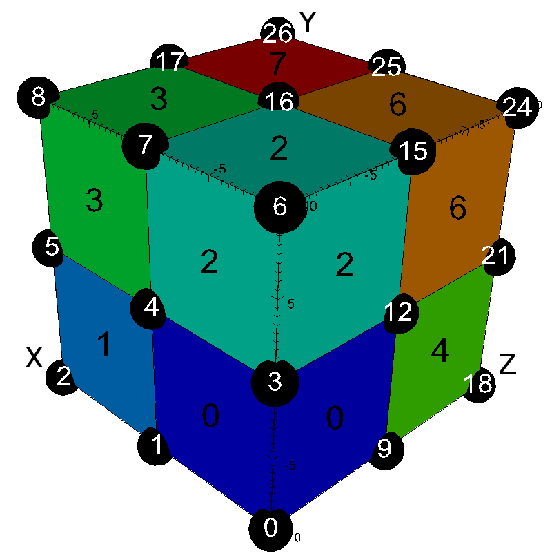
Pseudocolor plot of basic (mesh type ‘hexs’)

Wedges

• Usage Example

// create container node
Node mesh;
// generate simple explicit wedge-based 3d 'basic' mesh
conduit::blueprint::mesh::examples::basic("wedges", 3, 3, 3, mesh);
// print out results
std::cout << mesh.to_yaml() << std::endl;

• Result

coordsets: 
  coords: 
    type: "explicit"
    values: 
      x: [-10.0, 0.0, 10.0, -10.0, 0.0, 10.0, -10.0, 0.0, 10.0, -10.0, 0.0, 10.0, -10.0, 0.0, 10.0, -10.0, 0.0, 10.0, -10.0, 0.0, 10.0, -10.0, 0.0, 10.0, -10.0, 0.0, 10.0]
      y: [-10.0, -10.0, -10.0, 0.0, 0.0, 0.0, 10.0, 10.0, 10.0, -10.0, -10.0, -10.0, 0.0, 0.0, 0.0, 10.0, 10.0, 10.0, -10.0, -10.0, -10.0, 0.0, 0.0, 0.0, 10.0, 10.0, 10.0]
      z: [-10.0, -10.0, -10.0, -10.0, -10.0, -10.0, -10.0, -10.0, -10.0, 0.0, 0.0, 0.0, 0.0, 0.0, 0.0, 0.0, 0.0, 0.0, 10.0, 10.0, 10.0, 10.0, 10.0, 10.0, 10.0, 10.0, 10.0]
topologies: 
  mesh: 
    type: "unstructured"
    coordset: "coords"
    elements: 
      shape: "wedge"
      connectivity: [0, 1, 4, 9, 10, 13, 0, 3, 4, 9, 12, 13, 1, 2, 5, 10, 11, 14, 1, 4, 5, 10, 13, 14, 3, 4, 7, 12, 13, 16, 3, 6, 7, 12, 15, 16, 4, 5, 8, 13, 14, 17, 4, 7, 8, 13, 16, 17, 9, 10, 13, 18, 19, 22, 9, 12, 13, 18, 21, 22, 10, 11, 14, 19, 20, 23, 10, 13, 14, 19, 22, 23, 12, 13, 16, 21, 22, 25, 12, 15, 16, 21, 24, 25, 13, 14, 17, 22, 23, 26, 13, 16, 17, 22, 25, 26]
fields: 
  field: 
    association: "element"
    topology: "mesh"
    volume_dependent: "false"
    values: [0.0, 1.0, 2.0, 3.0, 4.0, 5.0, 6.0, 7.0, 8.0, 9.0, 10.0, 11.0, 12.0, 13.0, 14.0, 15.0]

• Visual

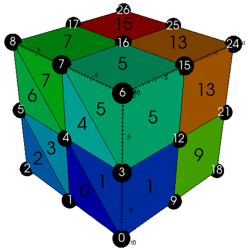
Pseudocolor plot of basic (mesh type ‘wedges’)

Pyramids

• Usage Example

// create container node
Node mesh;
// generate simple explicit pyramid-based 3d 'basic' mesh
conduit::blueprint::mesh::examples::basic("pyramids", 3, 3, 3, mesh);
// print out results
std::cout << mesh.to_yaml() << std::endl;

• Result

coordsets: 
  coords: 
    type: "explicit"
    values: 
      x: [-10.0, 0.0, 10.0, -10.0, 0.0, 10.0, -10.0, 0.0, 10.0, -10.0, 0.0, 10.0, -10.0, 0.0, 10.0, -10.0, 0.0, 10.0, -10.0, 0.0, 10.0, -10.0, 0.0, 10.0, -10.0, 0.0, 10.0, -5.0, 5.0, -5.0, 5.0, -5.0, 5.0, -5.0, 5.0]
      y: [-10.0, -10.0, -10.0, 0.0, 0.0, 0.0, 10.0, 10.0, 10.0, -10.0, -10.0, -10.0, 0.0, 0.0, 0.0, 10.0, 10.0, 10.0, -10.0, -10.0, -10.0, 0.0, 0.0, 0.0, 10.0, 10.0, 10.0, -5.0, -5.0, 5.0, 5.0, -5.0, -5.0, 5.0, 5.0]
      z: [-10.0, -10.0, -10.0, -10.0, -10.0, -10.0, -10.0, -10.0, -10.0, 0.0, 0.0, 0.0, 0.0, 0.0, 0.0, 0.0, 0.0, 0.0, 10.0, 10.0, 10.0, 10.0, 10.0, 10.0, 10.0, 10.0, 10.0, -5.0, -5.0, -5.0, -5.0, 5.0, 5.0, 5.0, 5.0]
topologies: 
  mesh: 
    type: "unstructured"
    coordset: "coords"
    elements: 
      shape: "pyramid"
      connectivity: [0, 3, 4, 1, 27, 0, 1, 10, 9, 27, 1, 4, 13, 10, 27, 4, 3, 12, 13, 27, 3, 0, 9, 12, 27, 9, 10, 13, 12, 27, 1, 4, 5, 2, 28, 1, 2, 11, 10, 28, 2, 5, 14, 11, 28, 5, 4, 13, 14, 28, 4, 1, 10, 13, 28, 10, 11, 14, 13, 28, 3, 6, 7, 4, 29, 3, 4, 13, 12, 29, 4, 7, 16, 13, 29, 7, 6, 15, 16, 29, 6, 3, 12, 15, 29, 12, 13, 16, 15, 29, 4, 7, 8, 5, 30, 4, 5, 14, 13, 30, 5, 8, 17, 14, 30, 8, 7, 16, 17, 30, 7, 4, 13, 16, 30, 13, 14, 17, 16, 30, 9, 12, 13, 10, 31, 9, 10, 19, 18, 31, 10, 13, 22, 19, 31, 13, 12, 21, 22, 31, 12, 9, 18, 21, 31, 18, 19, 22, 21, 31, 10, 13, 14, 11, 32, 10, 11, 20, 19, 32, 11, 14, 23, 20, 32, 14, 13, 22, 23, 32, 13, 10, 19, 22, 32, 19, 20, 23, 22, 32, 12, 15, 16, 13, 33, 12, 13, 22, 21, 33, 13, 16, 25, 22, 33, 16, 15, 24, 25, 33, 15, 12, 21, 24, 33, 21, 22, 25, 24, 33, 13, 16, 17, 14, 34, 13, 14, 23, 22, 34, 14, 17, 26, 23, 34, 17, 16, 25, 26, 34, 16, 13, 22, 25, 34, 22, 23, 26, 25, 34]
fields: 
  field: 
    association: "element"
    topology: "mesh"
    volume_dependent: "false"
    values: [0.0, 1.0, 2.0, 3.0, 4.0, 5.0, 6.0, 7.0, 8.0, 9.0, 10.0, 11.0, 12.0, 13.0, 14.0, 15.0, 16.0, 17.0, 18.0, 19.0, 20.0, 21.0, 22.0, 23.0, 24.0, 25.0, 26.0, 27.0, 28.0, 29.0, 30.0, 31.0, 32.0, 33.0, 34.0, 35.0, 36.0, 37.0, 38.0, 39.0, 40.0, 41.0, 42.0, 43.0, 44.0, 45.0, 46.0, 47.0]

• Visual

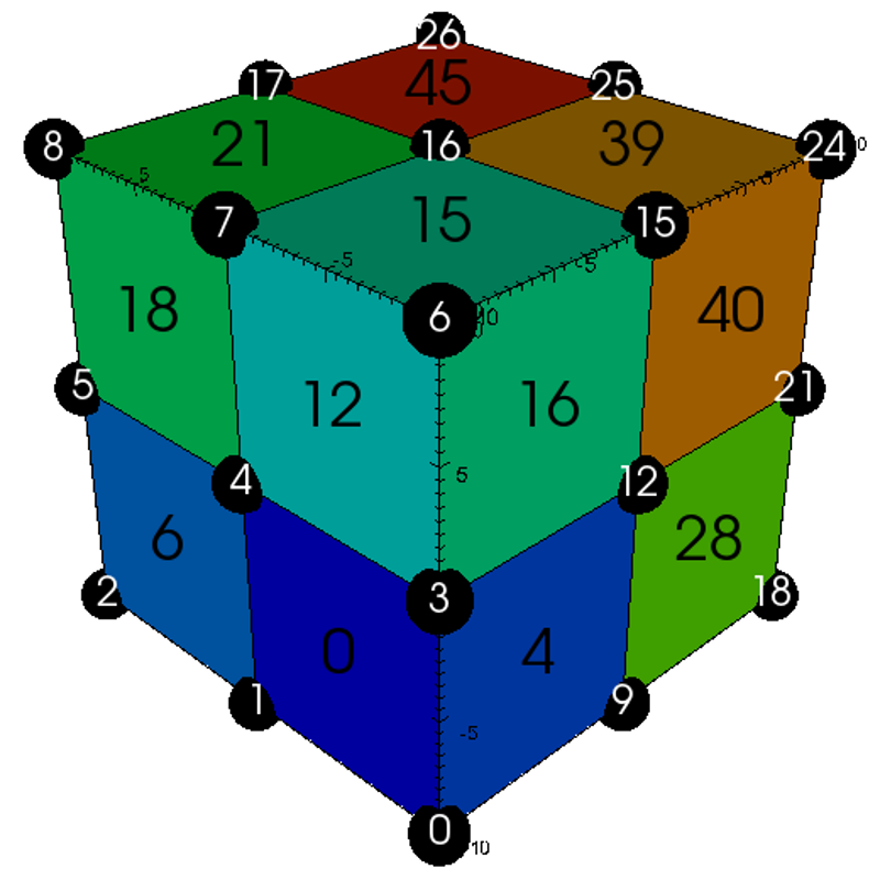
Pseudocolor plot of basic (mesh type ‘pyramids’)

Polyhedra

• Usage Example

// create container node
Node mesh;
// generate simple explicit poly-based 3d 'basic' mesh
conduit::blueprint::mesh::examples::basic("polyhedra", 3, 3, 3, mesh);
// print out results
std::cout << mesh.to_yaml() << std::endl;

• Result

coordsets: 
  coords: 
    type: "explicit"
    values: 
      x: [-10.0, 0.0, 10.0, -10.0, 0.0, 10.0, -10.0, 0.0, 10.0, -10.0, 0.0, 10.0, -10.0, 0.0, 10.0, -10.0, 0.0, 10.0, -10.0, 0.0, 10.0, -10.0, 0.0, 10.0, -10.0, 0.0, 10.0]
      y: [-10.0, -10.0, -10.0, 0.0, 0.0, 0.0, 10.0, 10.0, 10.0, -10.0, -10.0, -10.0, 0.0, 0.0, 0.0, 10.0, 10.0, 10.0, -10.0, -10.0, -10.0, 0.0, 0.0, 0.0, 10.0, 10.0, 10.0]
      z: [-10.0, -10.0, -10.0, -10.0, -10.0, -10.0, -10.0, -10.0, -10.0, 0.0, 0.0, 0.0, 0.0, 0.0, 0.0, 0.0, 0.0, 0.0, 10.0, 10.0, 10.0, 10.0, 10.0, 10.0, 10.0, 10.0, 10.0]
topologies: 
  mesh: 
    type: "unstructured"
    coordset: "coords"
    elements: 
      shape: "polyhedral"
      connectivity: [0, 1, 2, 3, 4, 5, 6, 7, 8, 9, 2, 10, 11, 3, 12, 13, 14, 15, 16, 9, 17, 18, 12, 19, 5, 20, 21, 22, 23, 24, 10, 25, 26, 27, 21, 28, 15, 22, 29, 30, 31, 32, 19, 27, 33, 34, 29, 35]
      sizes: [6, 6, 6, 6, 6, 6, 6, 6]
      offsets: [0, 6, 12, 18, 24, 30, 36, 42]
    subelements: 
      connectivity: [0, 3, 4, 1, 0, 1, 10, 9, 1, 4, 13, 10, 4, 3, 12, 13, 3, 0, 9, 12, 9, 10, 13, 12, 1, 4, 5, 2, 1, 2, 11, 10, 2, 5, 14, 11, 5, 4, 13, 14, 10, 11, 14, 13, 3, 6, 7, 4, 4, 7, 16, 13, 7, 6, 15, 16, 6, 3, 12, 15, 12, 13, 16, 15, 4, 7, 8, 5, 5, 8, 17, 14, 8, 7, 16, 17, 13, 14, 17, 16, 9, 10, 19, 18, 10, 13, 22, 19, 13, 12, 21, 22, 12, 9, 18, 21, 18, 19, 22, 21, 10, 11, 20, 19, 11, 14, 23, 20, 14, 13, 22, 23, 19, 20, 23, 22, 13, 16, 25, 22, 16, 15, 24, 25, 15, 12, 21, 24, 21, 22, 25, 24, 14, 17, 26, 23, 17, 16, 25, 26, 22, 23, 26, 25]
      sizes: [4, 4, 4, 4, 4, 4, 4, 4, 4, 4, 4, 4, 4, 4, 4, 4, 4, 4, 4, 4, 4, 4, 4, 4, 4, 4, 4, 4, 4, 4, 4, 4, 4, 4, 4, 4]
      shape: "polygonal"
      offsets: [0, 4, 8, 12, 16, 20, 24, 28, 32, 36, 40, 44, 48, 52, 56, 60, 64, 68, 72, 76, 80, 84, 88, 92, 96, 100, 104, 108, 112, 116, 120, 124, 128, 132, 136, 140]
fields: 
  field: 
    association: "element"
    topology: "mesh"
    volume_dependent: "false"
    values: [0.0, 1.0, 2.0, 3.0, 4.0, 5.0, 6.0, 7.0]

• Visual

Pseudocolor plot of basic (mesh type ‘polyhedra’)

braid

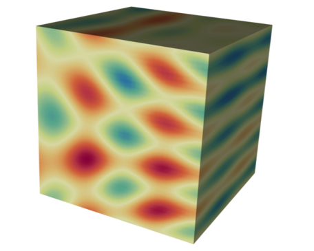
Pseudocolor plot of a 3D braid example braid field

The braid() generates example meshes that cover the range of coordinate sets and topologies supported by the Mesh Blueprint.

The example datasets include a vertex-centered scalar field braid, an element-centered scalar field radial and a vertex-centered vector field vel.

conduit::blueprint::mesh::examples::braid(const std::string &mesh_type,
                                          index_t nx,
                                          index_t ny,
                                          index_t nz,
                                          Node &res);

Here is a list of valid strings for the mesh_type argument:

Mesh Type	Description
uniform	2d or 3d uniform grid (implicit coords, implicit topology)
rectilinear	2d or 3d rectilinear grid (implicit coords, implicit topology)
structured	2d or 3d structured grid (explicit coords, implicit topology)
points	2d or 3d unstructured mesh of point elements (explicit coords, explicit topology)
points_implicit	2d or 3d point mesh (explicit coords, implicit topology)
lines	2d or 3d unstructured mesh of line elements (explicit coords, explicit topology)
tris	2d unstructured mesh of triangle elements (explicit coords, explicit topology)
quads	2d unstructured mesh of quadrilateral elements (explicit coords, explicit topology)
tets	3d unstructured mesh of tetrahedral elements (explicit coords, explicit topology)
hexs	3d unstructured mesh of hexahedral elements (explicit coords, explicit topology)
wedges	3d unstructured mesh of wedge elements (explicit coords, explicit topology)
pyramids	3d unstructured mesh of pyramid elements (explicit coords, explicit topology)
mixed_2d	2d unstructured mesh of mixed elements (explicit coords, explicit topology)
mixed	3d unstructured mesh of mixed elements (explicit coords, explicit topology)

nx, ny, nz specify the number of elements in the x, y, and z directions.

nz is ignored for 2d-only examples.

The resulting data is placed the Node res, which is passed in via reference.

spiral

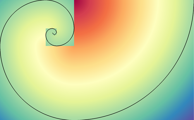
Pseudocolor and Contour plots of the spiral example dist field.

The spiral() function generates a multi-domain mesh composed of 2D square domains with the area of successive fibonacci numbers. The result estimates the Golden spiral.

The example dataset provides a vertex-centered scalar field dist that estimates the distance from each vertex to the Golden spiral.

conduit::blueprint::mesh::examples::spiral(conduit::index_t ndomains,
                                           Node &res);

ndomains specifies the number of domains to generate, which is also the number of entries from fibonacci sequence used.

The resulting data is placed the Node res, which is passed in via reference.

julia

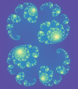
Pseudocolor plot of the julia example iter field

The julia() function creates a uniform grid that visualizes Julia set fractals.

The example dataset provides an element-centered scalar field iter that represents the number of iterations for each point tested or zero if not found in the set.

conduit::blueprint::mesh::examples::julia(index_t nx,
                                          index_t ny,
                                          float64 x_min,
                                          float64 x_max,
                                          float64 y_min,
                                          float64 y_max,
                                          float64 c_re,
                                          float64 c_im,
                                          Node &res);

nx, ny specify the number of elements in the x and y directions.

x_min, x_max, y_min, y_max specify the x and y extents.

c_re, c_im specify real and complex parts of the constant used.

The resulting data is placed the Node res, which is passed in via reference.

julia amr examples

We also provide examples that represent the julia set using AMR meshes. These functions provide concrete examples of the Mesh Blueprint nestset protocol for patch-based AMR meshes.

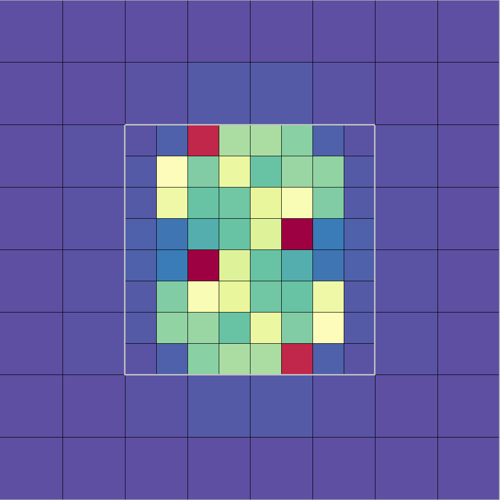
Pseudocolor, Mesh, and Domain Boundary plots of the julia_nestsets_simple example.

conduit::blueprint::mesh::examples::julia_nestsets_simple(float64 x_min,
                                                          float64 x_max,
                                                          float64 y_min,
                                                          float64 y_max,
                                                          float64 c_re,
                                                          float64 c_im,
                                                          Node &res);

julia_nestsets_simple provides a basic AMR example with two levels and one parent/child nesting relationship.

x_min, x_max, y_min, y_max specify the x and y extents.

c_re, c_im specify real and complex parts of the constant used.

The resulting data is placed the Node res, which is passed in via reference.

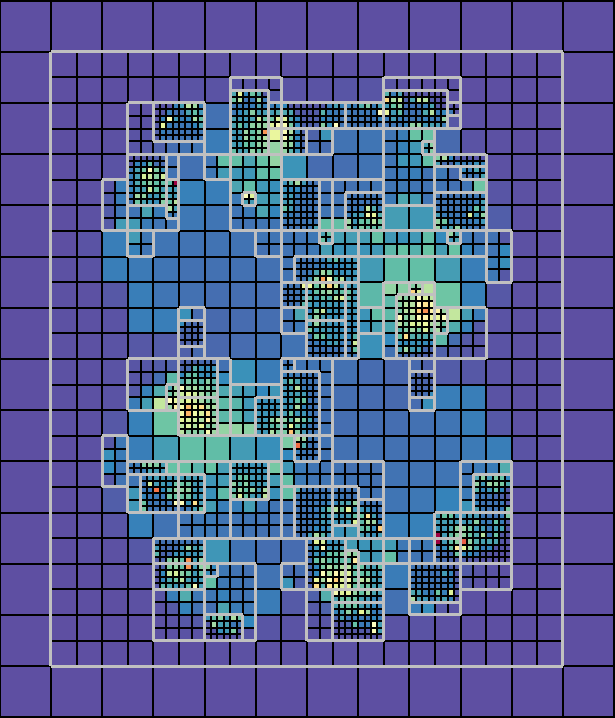
Pseudocolor, Mesh, and Domain Boundary plots of the julia_nestsets_complex example.

conduit::blueprint::mesh::examples::julia_nestsets_complex(index_t nx,
                                                           index_t ny,
                                                           float64 x_min,
                                                           float64 x_max,
                                                           float64 y_min,
                                                           float64 y_max,
                                                           float64 c_re,
                                                           float64 c_im,
                                                           index_t levels,
                                                           Node &res);

julia_nestsets_complex provides an AMR example that refines the mesh using more resolution in complex areas.

nx, ny specify the number of elements in the x and y directions.

x_min, x_max, y_min, y_max specify the x and y extents.

c_re, c_im specify real and complex parts of the constant used.

levels specifies the number of refinement levels to use.

The resulting data is placed the Node res, which is passed in via reference.

venn

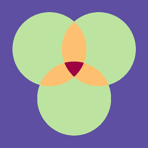
Pseudocolor plot of the venn example overlap field

The venn() function creates meshes that use three overlapping circle regions, demonstrating different ways to encode volume fraction based multi-material fields. The volume fractions are provided as both standard fields and using the Material sets (matsets) Blueprint. It also creates other fields related to overlap pattern.

conduit::blueprint::mesh::examples::venn(const std::string &matset_type,
                                         index_t nx,
                                         index_t ny,
                                         float64 radius,
                                         Node &res);

matset_type specifies the style of matset generated by the example.

Here is a list of valid strings for the matset_type argument:

Matset Type	Description
full	non-sparse volume fractions and matset values
sparse_by_material	sparse (material dominant) volume fractions and matset values
sparse_by_element	sparse (element dominant) volume fractions and matset values

nx, ny specify the number of elements in the x and y directions.

radius specifies the radius of the three circles.

The resulting data is placed the Node res, which is passed in via reference.

polytess

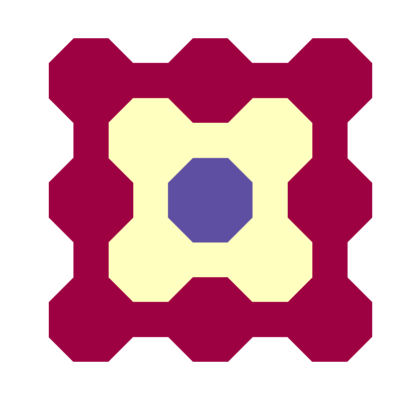
Pseudocolor plot of the polytess example level field, with nz = 1.

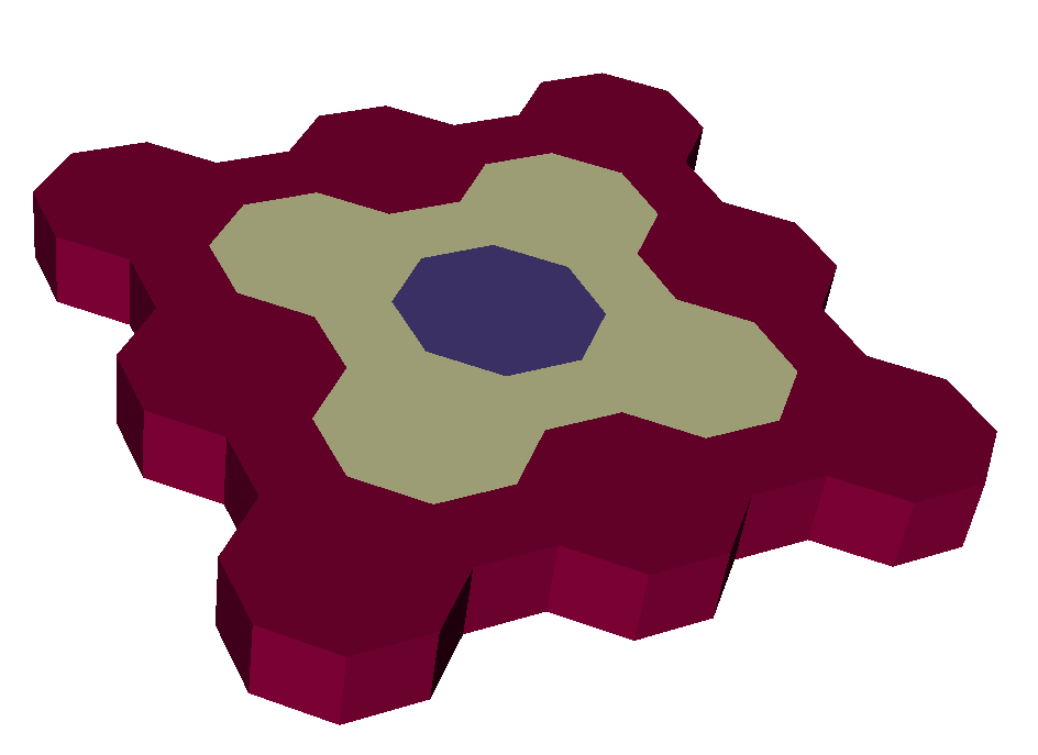
Pseudocolor plot of the polytess example level field, with nz = 2.

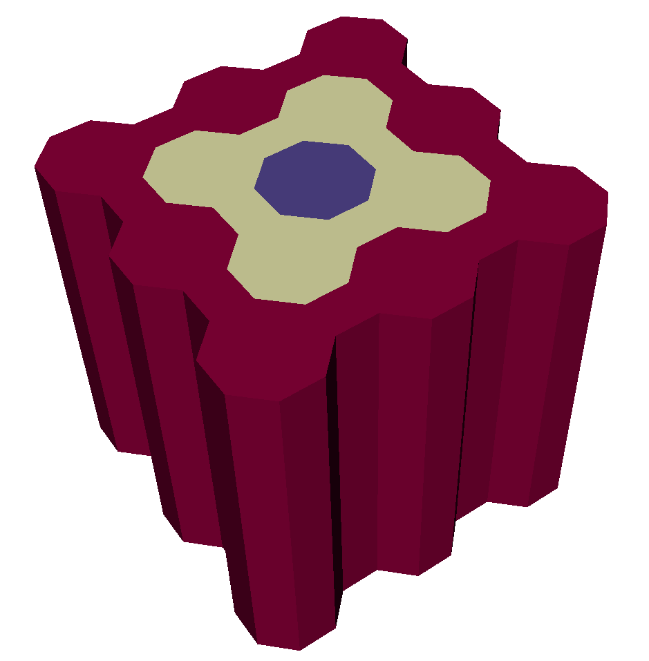
Pseudocolor plot of the polytess example level field, with nz = 10.

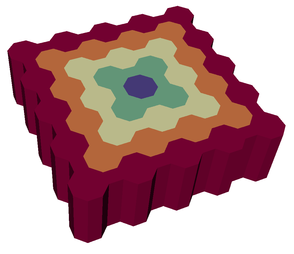
Pseudocolor plot of the polytess example level field, with nz = 6.

The polytess() function generates a polygonal tessellation in the 2D plane comprised of octagons and squares (known formally as a two-color truncated square tiling). This can be extended into 3D using the nz parameter, which, if greater than 1, will stack polytessalations on top of one another as follows: first, a polytess is placed into 3D space, and then a copy of it is placed into a plane parallel to the original. Then “walls” are added, and finally polyhedra are specified that use faces from the original polytess, the reflected copy, and the walls. An nz value of 3 or more will simply add layers to this setup, essentially stacking “sheets” of polytess on top of one another.

The scalar element-centered field level defined in the result mesh associates each element with its topological distance from the center of the tessellation.

conduit::blueprint::mesh::examples::polytess(index_t nlevels,
                                             index_t nz,
                                             Node &res);

nlevels specifies the number of tessellation levels/layers to generate. If this value is specified as 1 or less, only the central tessellation level (i.e. the octagon in the center of the geometry) will be generated in the result.

The resulting data is placed the Node res, which is passed in via reference.

polychain

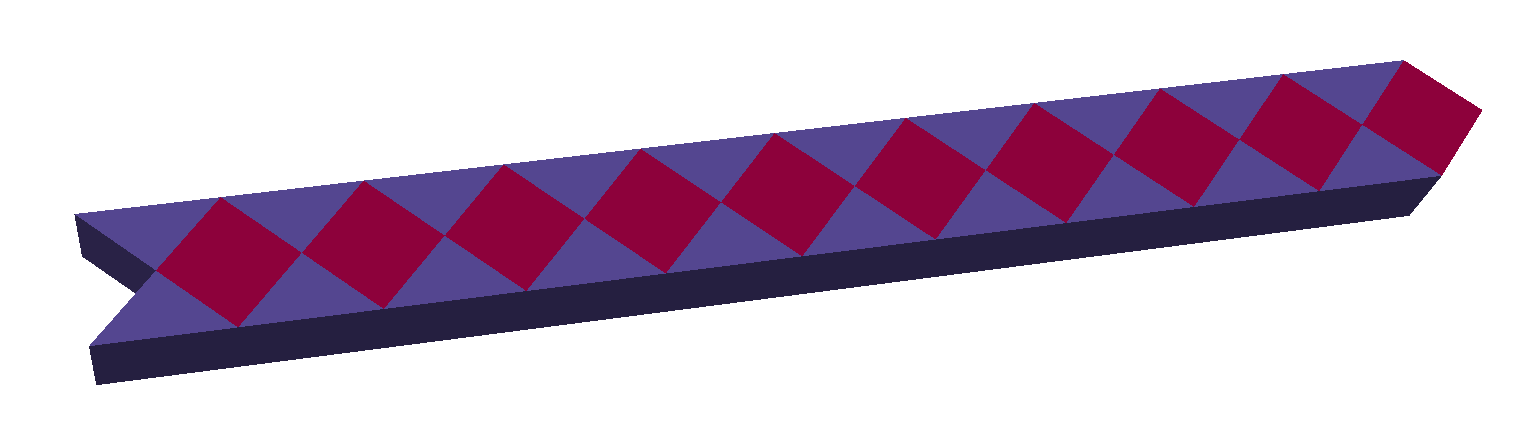
Pseudocolor plot of the polyhedral chain example chain field.

The polychain() function generates a chain of cubes and triangular prisms that extends diagonally.

The scalar element-centered field chain defined in the result mesh associates with each cube the value 0 and with each triangular prism the value 1.

conduit::blueprint::mesh::examples::polychain(const index_t length,
                                              Node &res);

length specifies how long the chain ought to be. The length is equal to the number of cubes and equal to half the number of prisms.

The resulting data is placed the Node res, which is passed in via reference.

tiled

The tiled() function repeats a tile (given as a 2D Blueprint topology) into a larger mesh composed of a regular square tiling of the supplied tile. If no topology is given, a default pattern consisting of quads is used. The output mesh can be either 2D or 3D. For 3D, supply a nz parameter greater than zero. Note that the input tile must consist of a homogeneous set of triangles or quads to extrude the tile into 3D since polyhedral output is not yet supported. The tiled() function produces a single domain comprised of a main mesh, a boundary mesh, and adjacency sets if the output mesh is to be part of a multi-domain dataset.

conduit::blueprint::mesh::examples::tiled(index_t nx,                   // number of tiles along x
                                          index_t ny,                   // number of tiles along y
                                          index_t nz,                   // number of elements along z (0 for 2D)
                                          conduit::Node &res,           // result container
                                          const conduit::Node &options);// options node

The tiled() function accepts a Conduit node containing options that influence how the mesh is generated. If the options contain a tile node that contains a 2D blueprint topology, the first supplied topology will be used to override the default tile pattern. The tile node may contain additional options. An important set of options define the left, right, bottom, and top sets of points within the supplied tile pattern. The values in the left option identify the list of points that define the left edge of the tile. These are indices into the coordset and the values should be in consecutive order along the edge. Opposite point sets must match. In other words, the left and right point sets must contain the same number of points and they need to proceed along their edges in the same order. The same is true of the bottom and top point sets. The optional translate/x and translate/y options determine the tile spacing. If the translation values are not given, they will be determined from the coordset extents.

The remaining options described are not part of the tile node. The reorder option indicates the type of point and element reordering that will be done. Reordering can improve cache-friendliness. The default is to reorder points and elements, using “kdtree” method. Passing “none” or an empty string will prevent reordering. The name of the mesh can be given by passing a meshname option string. Likewise, the name of the boundary mesh can be supplied using the boundarymeshname option. The output mesh topology will store its integer connectivity information as index_t by default. The precision of the integer output can turned to int32 by passing a datatype option containing the “int”, “int32”, “integer” strings.

The tiled() function also accepts options that simplify the task of generating mesh domains for a multi-domain dataset. The coordinate extents of the current mesh domain are given using the extents option, which contains 6 double values: {xmin, xmax, ymin, ymax, zmin, zmax}. The domains option contains a triple of {domainsI, domainsJ, domainsK} values that indicate how many divisions there are of the extents in the I,J,K dimensions. The product of these numbers determines the total number of domains. The domain option specifies a triple indicating the I,J,K domain id within the overall set of domains. This is used to help construct adjacency sets.

tile:
  # Define the tile
  coordsets:
    coords:
      type: explicit
      values:
        x: [0., 1., 2., 0., 1., 2., 0., 1., 2.]
        y: [0., 0.5, 0., 1., 1.5, 1., 2., 2.5, 2.]
  topologies:
    tile:
      type: unstructured
      coordset: coords
      elements:
        shape: tri
        connectivity: [0,1,4, 0,4,3, 1,2,5, 1,5,4, 3,4,7, 3,7,6, 4,5,8, 4,8,7]
  # Define the tile edges
  left: [0,3,6]
  right: [2,5,8]
  bottom: [0,1,2]
  top: [6,7,8]
  # Optional tile translation
  translate:
    x: 2.
    y: 2.
# Set some options that aid tiling.
reorder: kdtree
domain: [0,0,0]
domains: [2,2,2]
extents: [0., 0.5, 0., 0.5, 0., 0.5]

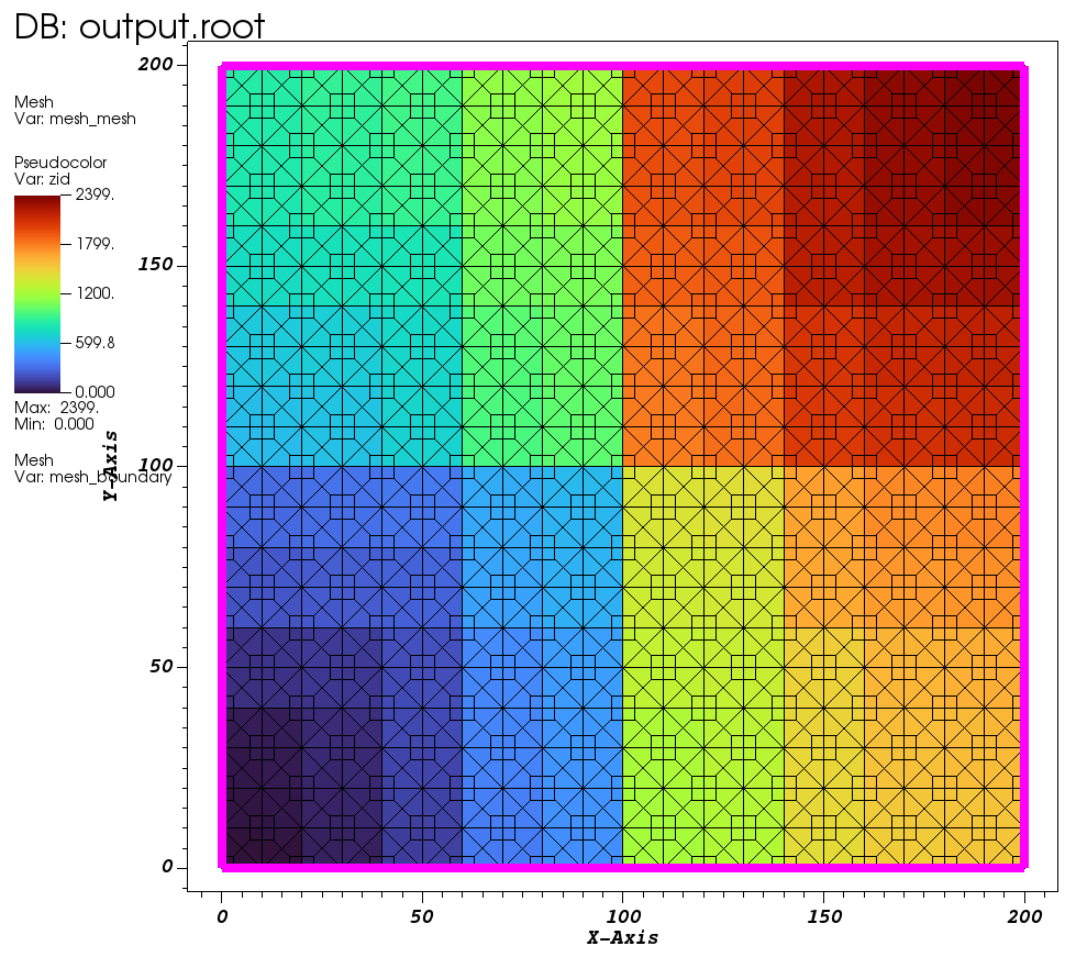
Pseudocolor plot of zoneid for default tile mesh that has been reordered.

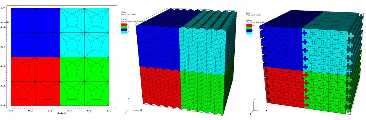
Subset plots of multi-domain datasets created using the tiled() function.

miscellaneous

This section doesn’t overview any specific example in the conduit::blueprint::mesh::examples namespace, but rather provides a few additional code samples to help with various common tasks. Each subsection covers a specific task and presents how it can be accomplished using a function or set of functions in Conduit and/or the Mesh Blueprint library.

Outputting Meshes for Visualization

Suppose that you have an arbitrary Blueprint mesh that you want to output from a running code and subsequently visualize using a visualization tool (e.g. VisIt). You can save your mesh to a set of files, using one of the following conduit::relay::io::blueprint library functions:

Save a mesh to disk:

conduit::relay::io::blueprint::write_mesh(const conduit::Node &mesh,
                                          const std::string &path);

Save a mesh to disk using a specific protocol:

conduit::relay::io::blueprint::write_mesh(const conduit::Node &mesh,
                                          const std::string &path,
                                          const std::string &protocol);

Save a mesh to disk using a specific protocol and options:

/// Options accepted via the `opts` Node argument:
///
///      file_style: "default", "root_only", "multi_file"
///            when # of domains == 1,  "default"   ==> "root_only"
///            else,                    "default"   ==> "multi_file"
///
///      suffix: "default", "cycle", "none"
///            when # of domains == 1,  "default"   ==> "none"
///            else,                    "default"   ==> "cycle"
///
///      mesh_name:  (used if present, default ==> "mesh")
///
///      number_of_files:  {# of files}
///            when "multi_file":
///                 <= 0, use # of files == # of domains
///                  > 0, # of files == number_of_files
///
conduit::relay::io::blueprint::write_mesh(const conduit::Node &mesh,
                                          const std::string &path,
                                          const std::string &protocol,
                                          const conduit::Node &opts);

Loading Meshes from Files

If you have a mesh written to a set of blueprint files, you can load them by passing the root file path to the following conduit::relay::io::blueprint library functions:

Load a mesh given a root file:

conduit::relay::io::blueprint::read_mesh(const std::string &root_file_path,
                                         conduit::Node &mesh);

Load a mesh given a root file and options:

/// Options accepted via the `opts` Node argument:
///
///      mesh_name: "{name}"
///          provide explicit mesh name, for cases where bp data includes
///           more than one mesh.
///
conduit::relay::io::blueprint::read_mesh(const std::string &root_file_path,
                                         const conduit::Node &opts,
                                         conduit::Node &mesh);

Complete Uniform Example

This snippet provides a complete C++ example that demonstrates:

• Describing a single-domain uniform mesh in a Conduit tree

• Verifying the tree conforms to the Mesh Blueprint

• Saving the result to a file that VisIt and Ascent Replay can open

// create a Conduit node to hold our mesh data
Node mesh;

// create the coordinate set
mesh["coordsets/coords/type"] = "uniform";
mesh["coordsets/coords/dims/i"] = 3;
mesh["coordsets/coords/dims/j"] = 3;
// add origin and spacing to the coordset (optional)
mesh["coordsets/coords/origin/x"] = -10.0;
mesh["coordsets/coords/origin/y"] = -10.0;
mesh["coordsets/coords/spacing/dx"] = 10.0;
mesh["coordsets/coords/spacing/dy"] = 10.0;

// add the topology
// this case is simple b/c it's implicitly derived from the coordinate set
mesh["topologies/topo/type"] = "uniform";
// reference the coordinate set by name
mesh["topologies/topo/coordset"] = "coords";

// add a simple element-associated field 
mesh["fields/ele_example/association"] =  "element";
// reference the topology this field is defined on by name
mesh["fields/ele_example/topology"] =  "topo";
// set the field values, for this case we have 4 elements
mesh["fields/ele_example/values"].set(DataType::float64(4));

float64 *ele_vals_ptr = mesh["fields/ele_example/values"].value();

for(int i=0;i<4;i++)
{
    ele_vals_ptr[i] = float64(i);
}

// add a simple vertex-associated field 
mesh["fields/vert_example/association"] =  "vertex";
// reference the topology this field is defined on by name
mesh["fields/vert_example/topology"] =  "topo";
// set the field values, for this case we have 9 vertices
mesh["fields/vert_example/values"].set(DataType::float64(9));

float64 *vert_vals_ptr = mesh["fields/vert_example/values"].value();

for(int i=0;i<9;i++)
{
    vert_vals_ptr[i] = float64(i);
}

// make sure we conform:
Node verify_info;
if(!blueprint::mesh::verify(mesh, verify_info))
{
    std::cout << "Verify failed!" << std::endl;
    verify_info.print();
}

// print out results
std::cout << mesh.to_yaml() << std::endl;

// save our mesh to a file that can be read by VisIt
//
// this will create the file: complete_uniform_mesh_example.root
// which includes the mesh blueprint index and the mesh data
conduit::relay::io::blueprint::save_mesh(mesh,
                                         "complete_uniform_mesh_example",
                                         "json");

Expressions (Derived Fields)

An expression is a mathematical formula which defines a new field in terms of other fields and/or other expressions. Expressions are specified in the expressions section of the Blueprint protocol. The expressions section is optional. When it exists, it is a peer to the fields section. It is a list of Objects of the form:

• expressions/expression/number_of_components

• expressions/expression/topology

• expressions/expression/definition

The number_of_components and topology entries are identical to their meaning as entries in the fields section.

The definition entry is string valued and holds the expression (e.g. mathematical formula) defining how the new field is computed. Blueprint does not interpret this string. It simply passes it along for downstream consumers that have the ability to interpret the string and perform the associated operations to compute the expression.

If the expected consumer is VisIt, data producers may wish to consult the Expressions chapter of the VisIt user’s manual. In addition, data producers should escape all names of fields or expressions by bracketing them in < and > characters. An example expressions entry in the index is

{
"fields":
{
  "braid":
  {

  },
  "radial":
  {

  }
},
"expressions":
{
  "scalar_expr":
  {
    "number_of_components": 1,
    "topology": "mesh",
    "definition": "<vector_expr>[1]"
  },
  "vector_expr":
  {
    "number_of_components": 2,
    "topology": "mesh",
    "definition": "{<braid>,recenter(<radial>,\"nodal\")}"
  }
}
}